1.11. Himmelblau’s function#
Himmelblau’s function is another famous mathematical function used as a benchmark problem in optimization. It’s named after David Mautner Himmelblau, who introduced it in 1972. The function is defined as follows:

Fig. 1.7 Himmelblau’s function Source: https://commons.wikimedia.org/wiki/File:Himmelblau_function.svg. Image by Morn the Gorn. Released to the public domain#
Although this function seems simpler in comparison to the Eggholder function, it draws interest as it is multi-modal, in other words, it has more than one global minimum. To be exact, the function has four global minima evaluating to 0, which can be found in the following locations:
x=3.0, y=2.0
x=−2.805118, y=3.131312
x=−3.779310, y=−3.283186
x=3.584458, y=−1.848126
Which can be despicted here:
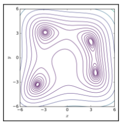
Fig. 1.8 Contour diagram of Himmelblau’s function Source: https://commons.wikimedia.org/wiki/File:Himmelblau_contour.svg. Image by: Nicoguaro. Licensed under Creative Commons CC BY 4.0: https://creativecommons.org/licenses/by/4.0/deed.en.#
Let’s break it down:
The Structure: Himmelblau’s function is made up of two polynomial terms, each squared and added together.
The Variables: The function depends on two variables, ( x ) and ( y ), which represent coordinates on a 2D plane.
The Squares: Each term in the function is squared. Squaring ensures that all parts of the function are positive, which can create multiple local minima and maxima.
The Constants: The numbers 11 and 7 in the function are constants.
The Summation: The squared terms are added together to form a single value, which represents the height of the function’s surface at a given point ( (x,y) ).
The Objective: The goal is to find the minimum value of the function, which corresponds to the lowest point on its surface.
Himmelblau’s function is particularly interesting because it has four identical local minima, each with a value of 0, and one global minimum also at 0. These minima are located at the points:
These points are like valleys in the landscape represented by the function, and finding them can be challenging due to the function’s complex structure with multiple hills and valleys.
In optimization, scientists and engineers use Himmelblau’s function to test and compare different optimization algorithms. The efficiency of an algorithm is measured by how quickly and accurately it can find the global minimum (the lowest point) of the function. If an algorithm can efficiently navigate the landscape of Himmelblau’s function to find the minima, it’s likely to perform well on other optimization problems too.
from deap import base
from deap import creator
from deap import tools
import random
import numpy as np
import matplotlib.pyplot as plt
import seaborn as sns
import elitism
def run_himmelblau_optimization_genetic(DIMENSIONS = 2, BOUND_LOW = -5.0, BOUND_UP = 5.0, POPULATION_SIZE = 300, P_CROSSOVER = 0.9, P_MUTATION = 0.5, MAX_GENERATIONS = 300, HALL_OF_FAME_SIZE = 30, CROWDING_FACTOR = 20.0, RANDOM_SEED = 42):
random.seed(RANDOM_SEED)
toolbox = base.Toolbox()
# define a single objective, minimizing fitness strategy:
creator.create("FitnessMin", base.Fitness, weights=(-1.0,))
# create the Individual class based on list:
creator.create("Individual", list, fitness=creator.FitnessMin)
# helper function for creating random float numbers uniformaly distributed within a given range [low, up]
# it assumes that the range is the same for every dimension
def randomFloat(low, up):
return [random.uniform(a, b) for a, b in zip([low] * DIMENSIONS, [up] * DIMENSIONS)]
# create an operator that randomly returns a float in the desired range and dimension:
toolbox.register("attr_float", randomFloat, BOUND_LOW, BOUND_UP)
# create the individual operator to fill up an Individual instance:
toolbox.register("individualCreator", tools.initIterate, creator.Individual, toolbox.attr_float)
# create the population operator to generate a list of individuals:
toolbox.register("populationCreator", tools.initRepeat, list, toolbox.individualCreator)
# Himmelblau function as the given individual's fitness:
def himmelblau(individual):
x = individual[0]
y = individual[1]
f = (x ** 2 + y - 11) ** 2 + (x + y ** 2 - 7) ** 2
return f, # return a tuple
toolbox.register("evaluate", himmelblau)
# genetic operators:
toolbox.register("select", tools.selTournament, tournsize=2)
toolbox.register("mate", tools.cxSimulatedBinaryBounded, low=BOUND_LOW, up=BOUND_UP, eta=CROWDING_FACTOR)
toolbox.register("mutate", tools.mutPolynomialBounded, low=BOUND_LOW, up=BOUND_UP, eta=CROWDING_FACTOR, indpb=1.0/DIMENSIONS)
# create initial population (generation 0):
population = toolbox.populationCreator(n=POPULATION_SIZE)
# prepare the statistics object:
stats = tools.Statistics(lambda ind: ind.fitness.values)
stats.register("min", np.min)
stats.register("avg", np.mean)
# define the hall-of-fame object:
hof = tools.HallOfFame(HALL_OF_FAME_SIZE)
# perform the Genetic Algorithm flow with elitism:
population, logbook = elitism.eaSimpleWithElitism(population, toolbox, cxpb=P_CROSSOVER, mutpb=P_MUTATION,
ngen=MAX_GENERATIONS, stats=stats, halloffame=hof, verbose=True)
# print info for best solution found:
best = hof.items[0]
print("-- Best Individual = ", best)
print("-- Best Fitness = ", best.fitness.values[0])
print("- Best solutions are:")
for i in range(HALL_OF_FAME_SIZE):
print(i, ": ", hof.items[i].fitness.values[0], " -> ", hof.items[i])
# extract statistics:
minFitnessValues, meanFitnessValues = logbook.select("min", "avg")
return minFitnessValues, meanFitnessValues, population
minFitnessValues_42, meanFitnessValues_42, population_42 = run_himmelblau_optimization_genetic(RANDOM_SEED=42)
# random with seed 13 for comparison:
minFitnessValues_13, meanFitnessValues_13, population_13 = run_himmelblau_optimization_genetic(RANDOM_SEED=13)
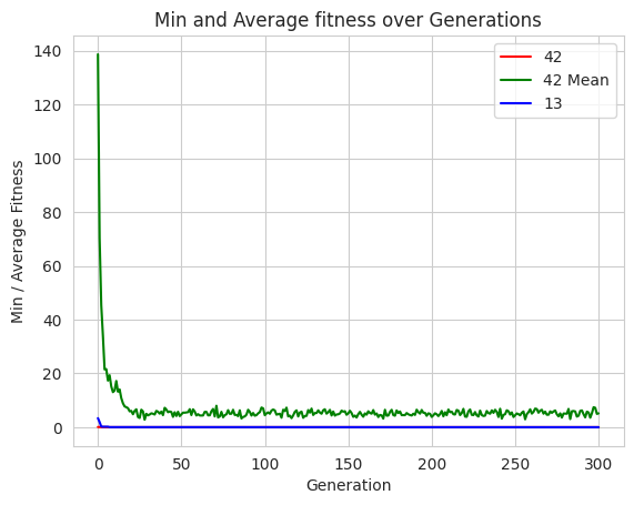
# plot statistics:
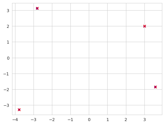
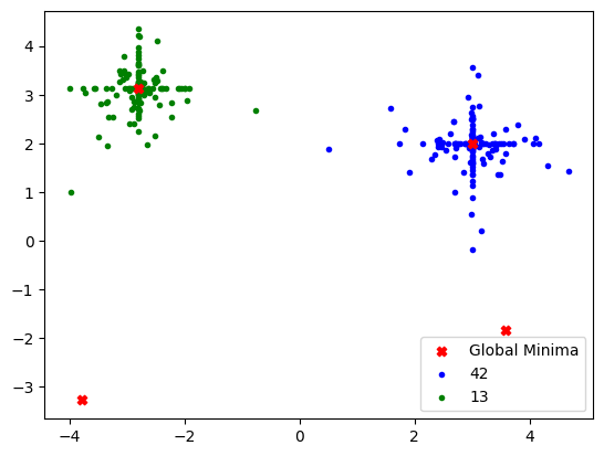
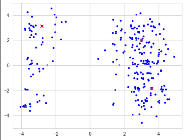
# plot solution locations on x-y plane:
plt.figure(1)
globalMinima = [[3.0, 2.0], [-2.805118, 3.131312], [-3.779310, -3.283186], [3.584458, -1.848126]]
plt.scatter(*zip(*globalMinima), marker='X', color='red', zorder=1)
plt.scatter(*zip(*population_42), marker='.', color='blue', zorder=0)
plt.scatter(*zip(*population_13), marker='.', color='green', zorder=0)
# Legends and labels.
plt.legend(['Global Minima', '42', '13'])
plt.figure(2)
sns.set_style("whitegrid")
plt.plot(minFitnessValues_42, color='red')
plt.plot(meanFitnessValues_42, color='green')
plt.plot(minFitnessValues_13, color='blue')
plt.xlabel('Generation')
plt.ylabel('Min / Average Fitness')
plt.title('Min and Average fitness over Generations')
# Legends.
plt.legend(['42', '42 Mean', '13'])
plt.show()
gen	nevals	min     	avg
0  	300   	0.077887	138.646
1  	256   	0.077887	70.3018
2  	261   	0.0549376	45.3529
3  	260   	0.0549376	34.0376
4  	253   	0.0421103	21.4902
5  	259   	0.00375114	21.5907
6  	255   	0.00163305	17.3338
7  	265   	0.00163305	19.3309
8  	252   	0.00163305	15.1737
9  	249   	0.000356589	13.0519
10 	258   	0.000356589	13.6612
11 	257   	0.00027667 	17.1779
12 	256   	0.00027667 	13.212
13 	255   	7.48096e-05	14.0379
14 	254   	7.48096e-05	10.8216
15 	261   	2.53197e-05	8.90194
16 	258   	2.53197e-05	7.73907
17 	262   	2.53197e-05	7.43993
18 	258   	2.53197e-05	7.086
19 	250   	7.19839e-06	5.91175
20 	252   	4.87197e-06	6.0666
21 	256   	2.2194e-06 	4.83019
22 	252   	1.41761e-06	6.06226
23 	260   	1.41761e-06	6.66497
24 	258   	1.30806e-06	3.77568
25 	256   	1.30806e-06	3.44466
26 	264   	6.64878e-08	6.49944
27 	255   	6.64878e-08	5.88264
28 	257   	6.64878e-08	2.79407
29 	263   	6.64878e-08	4.97824
30 	252   	6.64878e-08	4.42222
31 	246   	6.09978e-08	4.7264
32 	260   	6.09978e-08	5.17458
33 	255   	6.09978e-08	5.00506
34 	248   	5.92724e-08	4.71614
35 	253   	4.92809e-08	6.06632
36 	250   	4.92809e-08	5.75887
37 	259   	4.92809e-08	5.04934
38 	262   	6.7185e-09 	5.79557
39 	255   	6.7185e-09 	4.49387
40 	261   	6.7185e-09 	7.20528
41 	261   	6.7185e-09 	6.55486
42 	248   	6.7185e-09 	5.58253
43 	254   	6.7185e-09 	5.84513
44 	254   	6.7185e-09 	5.65996
45 	255   	5.98006e-09	3.85545
46 	252   	5.83204e-09	5.57192
47 	248   	4.37779e-09	4.175
48 	254   	4.37779e-09	5.74221
49 	255   	4.37779e-09	4.14253
50 	250   	3.54443e-09	4.78216
51 	266   	3.35848e-09	5.43377
52 	265   	8.84248e-10	5.40311
53 	252   	8.84248e-10	5.49593
54 	259   	8.84248e-10	5.59
55 	260   	8.84248e-10	6.70795
56 	257   	7.94254e-11	4.51569
57 	262   	7.94254e-11	6.6488
58 	257   	3.91143e-11	5.81699
59 	253   	3.91143e-11	4.35297
60 	253   	3.91143e-11	4.84955
61 	258   	3.73926e-11	4.36845
62 	254   	3.73926e-11	4.34962
63 	263   	6.59053e-12	4.37778
64 	257   	6.59053e-12	5.70127
65 	252   	5.27567e-12	5.70112
66 	245   	5.27567e-12	4.41927
67 	254   	5.27567e-12	4.43039
68 	258   	5.27567e-12	5.94242
69 	253   	4.15001e-12	6.78561
70 	254   	4.14926e-12	4.00583
71 	259   	4.14926e-12	7.96415
72 	259   	4.14926e-12	3.64832
73 	257   	4.14924e-12	4.02725
74 	258   	3.82499e-12	5.71551
75 	255   	3.71594e-12	3.70308
76 	260   	3.68593e-12	4.48195
77 	258   	3.68593e-12	4.80197
78 	261   	3.68593e-12	6.34867
79 	259   	3.60916e-12	4.97059
80 	254   	3.47847e-12	5.02246
81 	259   	3.47802e-12	6.47276
82 	262   	3.43591e-12	4.55467
83 	259   	3.43591e-12	4.63276
84 	252   	9.90117e-13	4.12008
85 	266   	4.60997e-13	6.28692
86 	254   	4.48486e-13	3.25242
87 	253   	4.02874e-13	3.813
88 	263   	4.02874e-13	4.02812
89 	244   	2.74599e-14	4.65641
90 	263   	2.74599e-14	6.48003
91 	259   	2.74599e-14	5.68404
92 	250   	2.6433e-14 	4.33109
93 	253   	2.6433e-14 	5.2835
94 	260   	2.46705e-14	4.28592
95 	266   	8.80552e-15	4.50037
96 	255   	6.26147e-15	5.16448
97 	261   	6.26147e-15	5.62274
98 	253   	6.26147e-15	7.30574
99 	263   	6.26147e-15	7.00746
100	255   	5.2393e-15 	4.47544
101	245   	4.75521e-15	5.12811
102	263   	4.46882e-15	5.52925
103	257   	4.46882e-15	4.99727
104	261   	4.2743e-15 	6.20864
105	254   	4.2743e-15 	6.55723
106	254   	4.2743e-15 	6.26547
107	257   	4.2743e-15 	4.66188
108	256   	4.2743e-15 	4.86191
109	253   	4.2743e-15 	5.00868
110	258   	4.2606e-15 	3.53641
111	259   	4.2606e-15 	6.48986
112	260   	4.18844e-15	5.99779
113	258   	1.2422e-15 	7.27412
114	263   	6.88896e-16	4.03056
115	253   	6.88896e-16	4.29077
116	245   	6.88896e-16	3.37854
117	262   	6.88896e-16	4.38584
118	257   	6.88896e-16	5.71372
119	251   	6.88563e-16	6.27232
120	253   	6.88563e-16	4.00742
121	258   	6.88563e-16	5.4352
122	258   	6.44992e-16	5.80938
123	254   	6.44992e-16	3.50288
124	258   	6.44992e-16	4.1607
125	262   	6.00234e-16	4.2262
126	260   	5.99939e-16	6.38462
127	255   	5.0302e-16 	5.42886
128	259   	4.71991e-16	6.92739
129	261   	4.71991e-16	4.55161
130	264   	4.71991e-16	5.27377
131	254   	4.71991e-16	5.26929
132	255   	4.26631e-16	6.26138
133	257   	1.51201e-17	5.44689
134	257   	1.51201e-17	5.01166
135	256   	1.51201e-17	6.2964
136	260   	1.51201e-17	6.67106
137	263   	1.51201e-17	5.04854
138	258   	1.51201e-17	5.56134
139	254   	1.51201e-17	6.43982
140	254   	1.48309e-17	4.36226
141	251   	1.16021e-17	5.83615
142	263   	1.16021e-17	4.2999
143	259   	1.12847e-17	4.74417
144	255   	8.27431e-18	4.79704
145	256   	8.27431e-18	5.11907
146	260   	8.27431e-18	6.16718
147	259   	8.26457e-18	5.76731
148	261   	8.26457e-18	5.94955
149	255   	5.68786e-18	4.61941
150	255   	3.8959e-18 	5.16448
151	258   	2.10357e-18	6.10652
152	261   	1.88468e-18	5.25709
153	258   	1.88468e-18	3.84778
154	255   	1.67776e-18	4.32516
155	259   	1.67776e-18	3.61752
156	253   	1.05342e-18	4.86505
157	260   	1.05342e-18	5.69881
158	251   	1.05342e-18	4.65244
159	256   	1.05342e-18	3.90631
160	259   	8.62071e-19	5.14928
161	259   	8.62071e-19	4.64952
162	255   	8.62071e-19	5.91489
163	262   	7.74407e-19	5.28551
164	260   	7.74407e-19	5.03704
165	251   	7.74407e-19	6.37295
166	258   	7.74407e-19	4.65555
167	258   	7.44463e-19	5.121
168	261   	7.44463e-19	3.79476
169	261   	7.44463e-19	4.55875
170	253   	6.61489e-19	4.39674
171	263   	6.61489e-19	3.19968
172	262   	6.28569e-19	6.48092
173	258   	6.15509e-19	4.28257
174	257   	6.15509e-19	4.35274
175	251   	6.15509e-19	5.69152
176	251   	6.15509e-19	6.46196
177	258   	6.15509e-19	4.5042
178	264   	6.15509e-19	4.28497
179	252   	4.88245e-19	6.24239
180	255   	4.88245e-19	5.24948
181	257   	4.88161e-19	5.8414
182	242   	4.03453e-19	4.49829
183	253   	3.76881e-19	4.48822
184	251   	1.35374e-19	4.49499
185	257   	1.34988e-19	5.26963
186	249   	1.31563e-19	4.80943
187	251   	5.55449e-20	4.53116
188	252   	5.55449e-20	4.35748
189	255   	5.55449e-20	5.01843
190	259   	5.55449e-20	4.58301
191	260   	5.55449e-20	6.50166
192	257   	5.55449e-20	5.60903
193	253   	3.72329e-20	5.0519
194	259   	3.72329e-20	6.40786
195	258   	3.72329e-20	5.38253
196	253   	3.71331e-20	5.33413
197	255   	3.71331e-20	4.24701
198	260   	3.71331e-20	5.15569
199	246   	3.71331e-20	4.97763
200	251   	3.11769e-20	3.8249
201	256   	3.11517e-20	4.43029
202	257   	3.09194e-20	5.17344
203	256   	2.91647e-20	4.81181
204	253   	2.84143e-20	4.1455
205	264   	2.49659e-20	4.88526
206	265   	2.32798e-20	6.04405
207	257   	2.32798e-20	4.05233
208	259   	2.32798e-20	5.56362
209	257   	8.71822e-21	4.47029
210	255   	8.61706e-21	6.56248
211	254   	8.61706e-21	5.5802
212	254   	8.61706e-21	5.76192
213	258   	8.36642e-21	4.82376
214	255   	5.57846e-21	4.73494
215	257   	3.95388e-21	6.41342
216	265   	3.61458e-21	6.15599
217	256   	2.43816e-21	4.51296
218	249   	2.43816e-21	5.26496
219	253   	2.43816e-21	6.82017
220	257   	2.43816e-21	3.95613
221	257   	2.43816e-21	3.88237
222	255   	2.43294e-21	5.90369
223	250   	2.38002e-21	6.57657
224	261   	2.07038e-21	4.6117
225	260   	2.07038e-21	4.50432
226	260   	1.20233e-21	5.63666
227	255   	1.19992e-21	4.41436
228	261   	1.19992e-21	3.97916
229	253   	1.19992e-21	6.17465
230	255   	1.19992e-21	4.52634
231	251   	1.19992e-21	4.18371
232	251   	1.17164e-21	4.31206
233	258   	1.17092e-21	6.02729
234	257   	1.17067e-21	5.26325
235	257   	1.16985e-21	5.01923
236	251   	1.15866e-21	6.26461
237	262   	1.12613e-21	5.34563
238	255   	7.63154e-22	6.4752
239	261   	5.93704e-22	5.7139
240	264   	5.93704e-22	3.81185
241	259   	5.93704e-22	6.86897
242	259   	5.92816e-22	3.18017
243	253   	5.92816e-22	4.56788
244	258   	5.92816e-22	4.83256
245	262   	5.92816e-22	6.29087
246	256   	5.75856e-22	5.94374
247	258   	5.75856e-22	4.69616
248	259   	5.75723e-22	5.50925
249	259   	6.3192e-23 	3.80087
250	259   	6.3192e-23 	4.41893
251	254   	6.3192e-23 	5.11537
252	258   	6.3192e-23 	4.86276
253	256   	6.3192e-23 	4.42574
254	253   	6.3192e-23 	5.3933
255	257   	6.08675e-23	5.84683
256	254   	6.08675e-23	2.948
257	261   	4.66027e-23	4.85923
258	266   	4.66027e-23	5.58709
259	258   	4.66027e-23	6.65547
260	254   	4.66027e-23	5.06172
261	256   	4.66027e-23	5.69355
262	262   	4.64348e-23	6.90995
263	254   	4.63872e-23	6.74979
264	256   	4.62394e-23	5.39876
265	256   	4.5475e-23 	6.16086
266	265   	4.5475e-23 	6.47227
267	253   	4.5475e-23 	5.04053
268	262   	4.5475e-23 	5.78258
269	255   	4.54412e-23	4.65128
270	264   	4.54412e-23	4.65313
271	261   	4.54412e-23	5.89047
272	260   	4.54412e-23	5.33603
273	261   	4.54412e-23	5.86113
274	250   	4.54412e-23	6.23454
275	252   	4.53438e-23	4.80711
276	251   	3.92798e-23	4.05758
277	260   	3.92641e-23	5.14986
278	253   	3.87712e-23	3.58922
279	256   	3.86246e-23	5.09143
280	246   	8.08865e-24	5.05197
281	257   	8.08865e-24	5.02208
282	253   	8.08865e-24	6.80142
283	251   	7.55373e-24	3.03274
284	263   	7.55373e-24	5.9319
285	254   	7.12276e-24	6.01458
286	254   	7.12276e-24	5.86623
287	256   	6.94241e-24	3.94701
288	261   	6.66183e-24	4.25718
289	260   	6.64995e-24	6.06468
290	248   	6.64995e-24	6.25063
291	251   	6.23736e-24	4.83061
292	248   	6.23736e-24	3.67227
293	263   	5.38278e-24	5.77907
294	260   	5.38278e-24	5.48787
295	255   	5.38278e-24	3.54449
296	248   	5.38278e-24	5.2204
297	260   	4.68039e-24	7.43367
298	251   	2.10797e-24	7.20637
299	253   	2.10797e-24	4.95986
300	257   	2.10797e-24	5.14909
-- Best Individual =  [2.9999999999998224, 2.000000000000362]
-- Best Fitness =  2.1079657119389998e-24
- Best solutions are:
0 :  2.1079657119389998e-24  ->  [2.9999999999998224, 2.000000000000362]
1 :  2.2357990439082543e-24  ->  [2.9999999999998224, 2.000000000000376]
2 :  2.3262466798572746e-24  ->  [3.000000000000002, 2.0000000000003686]
3 :  2.4863917545043818e-24  ->  [3.0000000000000235, 2.0000000000003673]
4 :  2.6850837284242085e-24  ->  [3.0000000000000444, 2.000000000000367]
5 :  2.969177783943262e-24  ->  [3.0000000000000644, 2.000000000000371]
6 :  4.277800995813578e-24  ->  [2.999999999999644, 2.0000000000003486]
7 :  4.308471907808571e-24  ->  [2.999999999999644, 2.0000000000003553]
8 :  4.542254781375344e-24  ->  [2.999999999999632, 2.0000000000003553]
9 :  4.608443366767008e-24  ->  [2.99999999999963, 2.000000000000362]
10 :  4.680387481323164e-24  ->  [2.9999999999996265, 2.000000000000362]
11 :  4.706675482128749e-24  ->  [2.9999999999996265, 2.0000000000003673]
12 :  4.8397973376066054e-24  ->  [2.9999999999998224, 2.000000000000581]
13 :  5.263674390087201e-24  ->  [2.999999999999598, 2.0000000000003553]
14 :  5.336940635520508e-24  ->  [2.9999999999995963, 2.000000000000362]
15 :  5.382780553861996e-24  ->  [2.999999999999594, 2.000000000000362]
16 :  5.443774490192779e-24  ->  [2.9999999999995914, 2.000000000000362]
17 :  5.752484950259254e-24  ->  [2.999999999999999, 2.000000000000582]
18 :  5.771079190656219e-24  ->  [3.0, 2.0000000000005826]
19 :  5.787651580553102e-24  ->  [3.0, 2.0000000000005835]
20 :  5.843784555985913e-24  ->  [3.000000000000001, 2.0000000000005858]
21 :  5.8451058980021585e-24  ->  [3.0000000000000107, 2.00000000000058]
22 :  5.849687602139682e-24  ->  [3.000000000000011, 2.00000000000058]
23 :  5.850208250337128e-24  ->  [3.000000000000002, 2.0000000000005853]
24 :  5.858535466052641e-24  ->  [3.000000000000002, 2.0000000000005858]
25 :  5.863536844191742e-24  ->  [3.0000000000000155, 2.0000000000005778]
26 :  5.866868992655396e-24  ->  [3.000000000000002, 2.000000000000586]
27 :  5.876855971715494e-24  ->  [3.000000000000011, 2.0000000000005813]
28 :  5.881636468801133e-24  ->  [3.000000000000003, 2.000000000000586]
29 :  5.885811120711563e-24  ->  [3.000000000000009, 2.000000000000583]
gen	nevals	min    	avg
0  	300   	3.35972	131.705
1  	256   	1.90913	81.8846
2  	255   	0.265975	48.9354
3  	255   	0.177752	34.6479
4  	254   	0.177752	23.392
5  	254   	0.177752	21.2792
6  	253   	0.177752	19.5267
7  	248   	0.0297201	19.8319
8  	253   	0.0297201	21.1444
9  	252   	0.0126402	17.6631
10 	254   	0.00985532	16.921
11 	252   	0.00191867	13.9612
12 	262   	0.000304058	15.7133
13 	252   	0.000304058	17.4744
14 	254   	0.000302592	14.7331
15 	261   	0.000302592	15.9097
16 	250   	0.000302592	15.5837
17 	248   	0.000302592	16.643
18 	264   	7.72395e-05	12.6406
19 	254   	7.72395e-05	16.6729
20 	248   	7.72395e-05	12.5159
21 	250   	5.24536e-05	11.0512
22 	257   	2.95871e-05	7.82117
23 	263   	2.95871e-05	10.4046
24 	262   	2.95871e-05	11.6654
25 	249   	9.34649e-06	11.0043
26 	259   	9.34649e-06	8.72941
27 	262   	9.30573e-06	7.16617
28 	263   	9.30573e-06	6.6125
29 	246   	4.77015e-06	7.0472
30 	259   	3.283e-06  	5.48927
31 	262   	2.45649e-06	7.83438
32 	266   	2.45649e-06	7.14255
33 	264   	1.34501e-06	7.79217
34 	256   	1.34501e-06	5.41112
35 	261   	7.97788e-07	8.89032
36 	259   	4.33689e-07	5.16245
37 	259   	4.33689e-07	6.92172
38 	260   	2.39012e-07	7.53679
39 	257   	2.39012e-07	5.83011
40 	260   	9.88903e-08	6.33394
41 	255   	9.88903e-08	7.56908
42 	260   	9.23784e-08	6.77589
43 	250   	9.23328e-08	6.51679
44 	252   	9.23328e-08	6.11241
45 	263   	9.02859e-08	10.4239
46 	251   	9.02692e-08	5.06779
47 	261   	2.80432e-08	8.88404
48 	259   	2.80432e-08	6.08482
49 	255   	7.83108e-10	5.33418
50 	255   	7.83108e-10	6.19978
51 	259   	7.83108e-10	5.16177
52 	257   	5.29982e-10	6.24265
53 	253   	5.29982e-10	7.42928
54 	260   	2.46922e-11	6.86718
55 	263   	2.46922e-11	8.75532
56 	256   	2.46922e-11	6.77635
57 	266   	2.46922e-11	8.66759
58 	266   	2.46922e-11	6.7659
59 	260   	1.8884e-11 	6.99401
60 	248   	1.8122e-11 	8.37096
61 	253   	1.20442e-11	6.71521
62 	259   	1.10707e-11	6.49011
63 	255   	1.10707e-11	5.35834
64 	251   	1.10707e-11	5.94653
65 	259   	1.37406e-12	6.33389
66 	251   	1.37406e-12	4.88938
67 	256   	1.04545e-12	5.77744
68 	262   	1.04545e-12	6.55077
69 	252   	1.04545e-12	9.31019
70 	253   	9.46575e-13	5.98201
71 	256   	9.46575e-13	7.04563
72 	253   	6.1396e-13 	6.34248
73 	260   	4.86526e-13	7.72951
74 	259   	4.64426e-13	3.82313
75 	260   	4.64426e-13	5.38473
76 	260   	3.51964e-13	8.12941
77 	258   	3.51964e-13	7.26752
78 	260   	3.51964e-13	6.66195
79 	252   	3.47942e-13	6.72551
80 	254   	2.90237e-13	7.35551
81 	250   	1.78021e-13	5.54314
82 	258   	1.78021e-13	6.58239
83 	259   	1.35224e-13	5.54233
84 	251   	1.35224e-13	7.05821
85 	254   	1.20844e-13	6.17379
86 	244   	1.20844e-13	6.77009
87 	261   	1.16697e-13	4.99726
88 	246   	6.65707e-14	8.44783
89 	261   	6.65707e-14	8.05532
90 	254   	6.65707e-14	7.65821
91 	251   	6.54001e-14	5.94519
92 	255   	6.54001e-14	6.06854
93 	249   	6.54001e-14	6.81517
94 	260   	6.54001e-14	4.99955
95 	255   	6.54001e-14	8.58214
96 	261   	6.48037e-14	9.59542
97 	254   	6.35391e-14	6.49097
98 	252   	6.35391e-14	8.2666
99 	257   	5.3458e-14 	8.73034
100	255   	5.32736e-14	7.00506
101	255   	5.26542e-14	6.67595
102	256   	5.13974e-14	3.38639
103	251   	5.13974e-14	6.15123
104	262   	4.01284e-15	7.48665
105	261   	4.01284e-15	7.32262
106	254   	4.01284e-15	6.21507
107	255   	4.01284e-15	7.19884
108	258   	2.59952e-15	5.34615
109	259   	1.88948e-15	5.03262
110	256   	1.78367e-15	6.51958
111	256   	4.05123e-16	8.124
112	260   	4.05123e-16	7.34357
113	244   	2.53543e-16	6.30368
114	263   	2.53543e-16	6.44179
115	259   	2.53543e-16	6.79736
116	259   	2.53543e-16	7.24266
117	259   	2.43527e-16	8.05971
118	253   	1.56581e-16	7.68931
119	257   	1.3426e-16 	8.51218
120	259   	1.3426e-16 	7.0655
121	251   	9.69829e-17	7.20644
122	252   	9.69829e-17	6.19084
123	262   	7.61345e-17	7.26602
124	251   	4.59978e-17	7.2042
125	259   	3.30461e-17	5.97054
126	264   	1.01725e-17	7.30965
127	252   	1.01389e-17	7.32988
128	247   	1.01389e-17	5.9945
129	262   	8.72297e-18	7.25127
130	256   	8.72297e-18	5.49504
131	258   	8.5969e-18 	5.60807
132	255   	8.5969e-18 	6.15457
133	262   	8.5969e-18 	5.87448
134	264   	6.56054e-18	5.53711
135	261   	5.92409e-18	6.97649
136	255   	4.98721e-18	6.42594
137	259   	4.84004e-18	4.98144
138	259   	3.88916e-18	6.75089
139	255   	3.88916e-18	8.08345
140	250   	3.88916e-18	7.06689
141	255   	3.88916e-18	6.79558
142	261   	3.88916e-18	6.01367
143	254   	3.88911e-18	7.65104
144	252   	3.88911e-18	5.90826
145	259   	3.88263e-18	8.44028
146	254   	3.87233e-18	7.95956
147	255   	3.58804e-18	8.09544
148	256   	3.58804e-18	7.51281
149	255   	3.58804e-18	7.99147
150	250   	2.24978e-18	6.89058
151	246   	2.24978e-18	7.82818
152	255   	2.24978e-18	5.33948
153	259   	2.24978e-18	6.26302
154	261   	2.16324e-18	5.30151
155	255   	2.11789e-18	6.95605
156	251   	2.09683e-18	7.17331
157	255   	2.09683e-18	11.8051
158	258   	1.99056e-18	6.59218
159	259   	1.99056e-18	6.03195
160	256   	1.94501e-18	7.54985
161	244   	1.94501e-18	4.34249
162	259   	1.94278e-18	3.89028
163	249   	1.94278e-18	5.88357
164	254   	1.94163e-18	5.96033
165	254   	1.93789e-18	6.22414
166	264   	1.93774e-18	5.72588
167	257   	1.93774e-18	6.91593
168	255   	1.93774e-18	7.04103
169	262   	1.93774e-18	7.31046
170	256   	1.93685e-18	8.22661
171	256   	1.91559e-18	6.91761
172	257   	1.90592e-18	7.34597
173	253   	5.0823e-19 	8.15843
174	262   	5.08025e-19	7.34421
175	262   	5.08025e-19	8.17275
176	256   	5.08025e-19	7.35377
177	262   	5.08025e-19	6.66899
178	257   	5.08025e-19	6.20248
179	254   	5.03051e-19	7.73716
180	255   	5.03051e-19	5.96824
181	257   	5.03051e-19	5.62636
182	259   	5.02954e-19	5.51099
183	254   	4.90419e-19	7.96762
184	251   	4.90419e-19	5.92094
185	255   	4.77754e-19	5.79599
186	251   	4.77595e-19	5.60364
187	265   	4.77585e-19	5.57927
188	249   	4.69989e-19	5.26512
189	255   	4.4437e-19 	5.07196
190	252   	4.09264e-19	6.27822
191	261   	4.09264e-19	5.74646
192	253   	4.09264e-19	9.74087
193	261   	4.06355e-19	6.80598
194	257   	4.06287e-19	6.71522
195	254   	4.0546e-19 	8.69995
196	255   	4.05167e-19	5.78905
197	250   	4.05167e-19	5.5018
198	253   	4.03857e-19	5.79457
199	254   	4.01593e-19	5.94866
200	251   	4.01593e-19	5.43499
201	249   	4.01593e-19	5.60869
202	253   	4.01593e-19	5.55366
203	247   	4.01593e-19	7.12702
204	257   	4.01593e-19	5.83665
205	255   	4.01589e-19	5.13001
206	255   	4.01589e-19	6.6097
207	259   	4.01238e-19	6.92252
208	258   	4.01156e-19	6.91222
209	256   	1.66989e-19	9.67415
210	248   	1.66989e-19	4.89261
211	260   	1.66989e-19	6.29826
212	259   	1.66749e-19	6.08951
213	259   	1.66749e-19	7.79635
214	260   	1.65285e-19	11.2637
215	263   	1.60196e-19	5.92847
216	258   	1.60196e-19	7.54245
217	243   	1.60196e-19	10.3501
218	259   	1.58667e-19	6.73682
219	256   	1.58667e-19	5.42762
220	259   	1.58667e-19	6.49389
221	263   	1.58667e-19	7.09991
222	251   	1.58667e-19	7.74504
223	255   	3.36858e-20	8.24159
224	258   	3.34878e-20	6.66071
225	260   	2.50129e-20	5.52411
226	252   	2.01406e-20	7.60913
227	257   	2.01406e-20	7.32581
228	254   	2.01406e-20	6.53484
229	257   	2.01406e-20	6.1063
230	261   	1.79566e-20	6.33952
231	255   	1.79566e-20	6.2471
232	260   	1.23683e-20	7.80874
233	256   	1.23683e-20	6.0578
234	248   	9.06692e-21	5.7183
235	258   	9.06692e-21	8.94956
236	247   	9.06692e-21	7.84818
237	256   	8.84508e-21	6.57898
238	260   	8.43193e-21	5.96024
239	257   	4.90363e-21	4.89623
240	251   	2.55674e-21	9.00758
241	256   	2.55674e-21	6.92852
242	261   	2.55674e-21	8.07276
243	251   	2.2828e-21 	6.9992
244	255   	2.2828e-21 	6.87258
245	258   	2.2828e-21 	5.06382
246	261   	2.2642e-21 	7.62386
247	250   	2.09475e-21	6.47462
248	252   	2.09475e-21	7.64577
249	256   	1.93027e-21	5.8076
250	245   	1.93027e-21	6.32176
251	255   	1.92338e-21	5.59437
252	255   	1.57729e-21	6.29478
253	258   	1.57729e-21	6.50337
254	262   	1.57729e-21	4.09771
255	256   	1.57729e-21	5.79421
256	255   	1.56906e-21	6.09066
257	262   	1.56906e-21	5.88922
258	256   	1.49091e-21	7.31839
259	256   	1.45303e-21	7.00971
260	257   	8.25205e-22	6.45142
261	252   	8.25205e-22	5.66843
262	254   	8.07696e-22	7.33748
263	254   	8.07696e-22	7.09352
264	260   	7.95836e-22	7.69431
265	255   	7.35414e-22	5.2441
266	251   	7.35414e-22	6.56227
267	249   	7.35414e-22	6.63325
268	248   	7.04587e-22	5.34459
269	252   	6.78952e-22	5.7212
270	259   	6.78952e-22	7.3687
271	260   	6.78952e-22	7.10475
272	258   	6.7624e-22 	7.79338
273	252   	5.97989e-22	8.34275
274	259   	5.97989e-22	9.81208
275	245   	5.97989e-22	7.36142
276	258   	5.97642e-22	6.93605
277	261   	5.9328e-22 	6.82679
278	258   	5.9328e-22 	7.48412
279	251   	4.37388e-22	9.4325
280	257   	4.37388e-22	7.72123
281	252   	3.67229e-22	7.10638
282	261   	3.67229e-22	5.32775
283	256   	3.67229e-22	7.55916
284	264   	3.65143e-22	5.68353
285	262   	3.65143e-22	8.26374
286	257   	2.024e-22  	6.13374
287	249   	6.72805e-23	6.40791
288	263   	6.72805e-23	8.1572
289	259   	6.72805e-23	6.92785
290	248   	6.72805e-23	7.0532
291	256   	6.66648e-23	7.03569
292	257   	6.66648e-23	4.84079
293	263   	6.59256e-23	7.85401
294	254   	6.59256e-23	5.99407
295	255   	6.59256e-23	6.31855
296	255   	6.58241e-23	6.59125
297	262   	6.42362e-23	6.09981
298	250   	6.42362e-23	7.71956
299	267   	5.95203e-23	7.82994
300	259   	5.91057e-23	5.10117
-- Best Individual =  [-2.805118086954073, 3.131312518250381]
-- Best Fitness =  5.910570309082829e-23
- Best solutions are:
0 :  5.910570309082829e-23  ->  [-2.805118086954073, 3.131312518250381]
1 :  5.952029051728901e-23  ->  [-2.805118086954078, 3.131312518250381]
2 :  6.302102486727553e-23  ->  [-2.805118086954135, 3.131312518250507]
3 :  6.357710554114031e-23  ->  [-2.805118086954136, 3.1313125182504598]
4 :  6.423617673934712e-23  ->  [-2.8051180869541352, 3.131312518250404]
5 :  6.429476464991698e-23  ->  [-2.8051180869541357, 3.131312518250404]
6 :  6.472412191910614e-23  ->  [-2.8051180869541406, 3.131312518250404]
7 :  6.487655508954381e-23  ->  [-2.805118086954143, 3.131312518250409]
8 :  6.495953063499858e-23  ->  [-2.805118086954143, 3.131312518250404]
9 :  6.496379995021763e-23  ->  [-2.805118086954146, 3.1313125182504202]
10 :  6.49854628595359e-23  ->  [-2.8051180869541392, 3.13131251825038]
11 :  6.50379820631619e-23  ->  [-2.8051180869541517, 3.1313125182504558]
12 :  6.505389496534202e-23  ->  [-2.805118086954148, 3.131312518250428]
13 :  6.508822540307633e-23  ->  [-2.8051180869541406, 3.131312518250382]
14 :  6.515460015964163e-23  ->  [-2.805118086954158, 3.131312518250507]
15 :  6.521394774326321e-23  ->  [-2.805118086954146, 3.131312518250404]
16 :  6.525470660851417e-23  ->  [-2.805118086954149, 3.1313125182504202]
17 :  6.526159494193856e-23  ->  [-2.8051180869541352, 3.1313125182503456]
18 :  6.531486829658995e-23  ->  [-2.8051180869541352, 3.1313125182503434]
19 :  6.535119691899719e-23  ->  [-2.8051180869541437, 3.131312518250382]
20 :  6.538869621098777e-23  ->  [-2.8051180869541437, 3.13131251825038]
21 :  6.541356110672034e-23  ->  [-2.805118086954158, 3.131312518250474]
22 :  6.554277967843916e-23  ->  [-2.805118086954154, 3.131312518250431]
23 :  6.555978120866849e-23  ->  [-2.805118086954146, 3.1313125182503825]
24 :  6.558073650975478e-23  ->  [-2.805118086954154, 3.1313125182504287]
25 :  6.582413480889529e-23  ->  [-2.8051180869541485, 3.1313125182503816]
26 :  6.592557601041947e-23  ->  [-2.8051180869541574, 3.131312518250428]
27 :  6.592876695278109e-23  ->  [-2.80511808695415, 3.131312518250382]
28 :  6.594497567780066e-23  ->  [-2.805118086954158, 3.1313125182504282]
29 :  6.596554049273887e-23  ->  [-2.805118086954155, 3.1313125182504096]
1.12. Using Niching and sharing to find Multiple Solutions#
1.12.1. TASK Complete the following method so that the following implementaiton: for optimizeHimmelblauSharing#
globalMaxima, population, hof, logbook, maxFitnessValues, meanFitnessValues = optimizeHimmelblauSharing()
# plot solution locations on x-y plane:
plt.figure(1)
plt.scatter(*zip(*globalMaxima), marker='x', color='red', zorder=1)
plt.scatter(*zip(*population), marker='.', color='blue', zorder=0) # plot solution locations on x-y plane:
# plot best solutions locations on x-y plane:
plt.figure(2)
plt.scatter(*zip(*globalMaxima), marker='x', color='red', zorder=1)
plt.scatter(*zip(*hof.items), marker='.', color='blue', zorder=0)
# extract statistics:
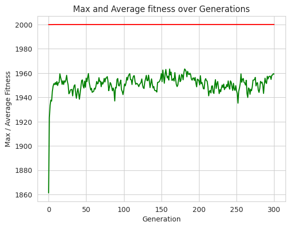
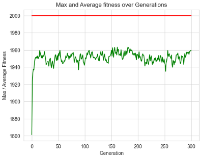
# plot statistics:
plt.figure(3)
sns.set_style("whitegrid")
plt.plot(maxFitnessValues, color='red')
plt.plot(meanFitnessValues, color='green')
plt.xlabel('Generation')
plt.ylabel('Max / Average Fitness')
plt.title('Max and Average fitness over Generations')
plt.show()
Use the following base code
1.12.2. Base Code#
from deap import base
from deap import creator
from deap import tools

import random
import numpy as np

import matplotlib.pyplot as plt
import seaborn as sns

import math
import elitism

def optimizeHimmelblauSharing(DIMENSIONS = 2, BOUND_LOW = -5.0, BOUND_UP = 5.0, POPULATION_SIZE = 300, P_CROSSOVER = 0.9, P_MUTATION = 0.5, MAX_GENERATIONS = 300, HALL_OF_FAME_SIZE = 30, CROWDING_FACTOR = 20.0, DISTANCE_THRESHOLD = 0.1, SHARING_EXTENT = 5.0, RANDOM_SEED = 42):

    random.seed(RANDOM_SEED)

    toolbox = base.Toolbox()

    # define a single objective, maximizing fitness strategy:
    creator.create("FitnessMax", base.Fitness, weights=(1.0,))

    # create the Individual class based on list:
    creator.create("Individual", list, fitness=creator.FitnessMax)


    # helper function for creating random float numbers uniformaly distributed within a given range [low, up]
    # it assumes that the range is the same for every dimension
    def randomFloat(low, up):
        return [random.uniform(a, b) for a, b in zip([low] * DIMENSIONS, [up] * DIMENSIONS)]

    # create an operator that randomly returns a float in the desired range and dimension:
    toolbox.register("attr_float", randomFloat, BOUND_LOW, BOUND_UP)

    # create the individual operator to fill up an Individual instance:
    toolbox.register("individualCreator", tools.initIterate, creator.Individual, toolbox.attr_float)

    # create the population operator to generate a list of individuals:
    toolbox.register("populationCreator", tools.initRepeat, list, toolbox.individualCreator)


    # 'Inverted' Himmelblau function as the given individual's fitness:
    def himmelblauInverted(individual):
        x = individual[0]
        y = individual[1]
        f = (x ** 2 + y - 11) ** 2 + (x + y ** 2 - 7) ** 2
        return 2000.0 - f,  # return a tuple

    toolbox.register("evaluate", himmelblauInverted)

    # TODO Cp,[;ete wraps the tools.selTournament() with fitness sharing
    # same signature as tools.selTournament()
    def selTournamentWithSharing(individuals, k, tournsize, fit_attr="fitness"):

        # get orig fitnesses:
        origFitnesses = [ind.fitness.values[0] for ind in individuals]

        # TODO Iterate over each individual, calculate the sharingSum as the sum of  (1 - distance / (SHARING_EXTENT * DISTANCE_THRESHOLD))  each time the distance is less than the treshhold
        # Distance calulcates as: math.sqrt(((individuals[i][0] - individuals[j][0]) ** 2) + ((individuals[i][1] - individuals[j][1]) ** 2))
        # apply sharing to each individual:
        for i in range(len(individuals)):
            sharingSum = 1


            # reduce fitness accordingly:
            individuals[i].fitness.values = origFitnesses[i] / sharingSum,

        # apply original tools.selTournament() using modified fitness:
        selected = tools.selTournament(individuals, k, tournsize, fit_attr)

        # retrieve original fitness:
        for i, ind in enumerate(individuals):
            ind.fitness.values = origFitnesses[i],

        return selected


    # TODO REWRITE Implement genetic operators: as:
    # - Tournament selection with sharing torunament size 2
    # - Simulated Binary Crossover (SBX) with eta = CROWDING_FACTOR
    # - Polynomial mutation with eta = CROWDING_FACTOR
    # toolbox.register("select", selTournamentWithSharing, tournsize=2)
    # toolbox.register("mate", tools.cxSimulatedBinaryBounded, low=BOUND_LOW, up=BOUND_UP, eta=CROWDING_FACTOR)
    # toolbox.register("mutate", tools.mutPolynomialBounded, low=BOUND_LOW, up=BOUND_UP, eta=CROWDING_FACTOR, indpb=1.0/DIMENSIONS)


    # create initial population (generation 0):
    population = toolbox.populationCreator(n=POPULATION_SIZE)

    # prepare the statistics object:
    stats = tools.Statistics(lambda ind: ind.fitness.values)
    stats.register("max", np.max)
    stats.register("avg", np.mean)

    # define the hall-of-fame object:
    hof = tools.HallOfFame(HALL_OF_FAME_SIZE)

    # perform the Genetic Algorithm flow with elitism:
    population, logbook = elitism.eaSimpleWithElitism(population, toolbox, cxpb=P_CROSSOVER, mutpb=P_MUTATION,
                                            ngen=MAX_GENERATIONS, stats=stats, halloffame=hof, verbose=True)

    # print info for best solution found:
    best = hof.items[0]
    print("-- Best Individual = ", best)
    print("-- Best Fitness = ", best.fitness.values[0])

    print("- Best solutions are:")
    for i in range(HALL_OF_FAME_SIZE):
        print(i, ": ", hof.items[i].fitness.values[0], " -> ", hof.items[i])

    globalMaxima = [[3.0, 2.0], [-2.805118, 3.131312], [-3.779310, -3.283186], [3.584458, -1.848126]]
    maxFitnessValues, meanFitnessValues = logbook.select("max", "avg")
    return globalMaxima, population, hof, logbook, maxFitnessValues, meanFitnessValues


if __name__ == "__main__":
    globalMaxima, population, hof, logbook, maxFitnessValues, meanFitnessValues = optimizeHimmelblauSharing()

    # plot solution locations on x-y plane:
    plt.figure(1)
    # TODO Rewrite the following code to plot the solutions and the global maxima
    # plt.scatter(*zip(*globalMaxima), marker='x', color='red', zorder=1)
    # plt.scatter(*zip(*population), marker='.', color='blue', zorder=0)    # plot solution locations on x-y plane:

    # plot best solutions locations on x-y plane:
    plt.figure(2)
    plt.scatter(*zip(*globalMaxima), marker='x', color='red', zorder=1)
    plt.scatter(*zip(*hof.items), marker='.', color='blue', zorder=0)

    # extract statistics:

    # TODO Rewrite plot statistics:
    plt.figure(3)
    sns.set_style("whitegrid")
    # plt.plot(maxFitnessValues, color='red')
    # plt.plot(meanFitnessValues, color='green')
    # plt.xlabel('Generation')
    # plt.ylabel('Max / Average Fitness')
    # plt.title('Max and Average fitness over Generations')

    plt.show()
1.12.3. Solution#
from deap import base
from deap import creator
from deap import tools

import random
import numpy as np

import matplotlib.pyplot as plt
import seaborn as sns

import math
import elitism

def optimizeHimmelblauSharing(DIMENSIONS = 2, BOUND_LOW = -5.0, BOUND_UP = 5.0, POPULATION_SIZE = 300, P_CROSSOVER = 0.9, P_MUTATION = 0.5, MAX_GENERATIONS = 300, HALL_OF_FAME_SIZE = 30, CROWDING_FACTOR = 20.0, DISTANCE_THRESHOLD = 0.1, SHARING_EXTENT = 5.0, RANDOM_SEED = 42):

    random.seed(RANDOM_SEED)

    toolbox = base.Toolbox()

    # define a single objective, maximizing fitness strategy:
    creator.create("FitnessMax", base.Fitness, weights=(1.0,))

    # create the Individual class based on list:
    creator.create("Individual", list, fitness=creator.FitnessMax)


    # helper function for creating random float numbers uniformaly distributed within a given range [low, up]
    # it assumes that the range is the same for every dimension
    def randomFloat(low, up):
        return [random.uniform(a, b) for a, b in zip([low] * DIMENSIONS, [up] * DIMENSIONS)]

    # create an operator that randomly returns a float in the desired range and dimension:
    toolbox.register("attr_float", randomFloat, BOUND_LOW, BOUND_UP)

    # create the individual operator to fill up an Individual instance:
    toolbox.register("individualCreator", tools.initIterate, creator.Individual, toolbox.attr_float)

    # create the population operator to generate a list of individuals:
    toolbox.register("populationCreator", tools.initRepeat, list, toolbox.individualCreator)


    # 'Inverted' Himmelblau function as the given individual's fitness:
    def himmelblauInverted(individual):
        x = individual[0]
        y = individual[1]
        f = (x ** 2 + y - 11) ** 2 + (x + y ** 2 - 7) ** 2
        return 2000.0 - f,  # return a tuple

    toolbox.register("evaluate", himmelblauInverted)

    # wraps the tools.selTournament() with fitness sharing
    # same signature as tools.selTournament()
    def selTournamentWithSharing(individuals, k, tournsize, fit_attr="fitness"):

        # get orig fitnesses:
        origFitnesses = [ind.fitness.values[0] for ind in individuals]

        # apply sharing to each individual:
        for i in range(len(individuals)):
            sharingSum = 1

            # iterate over all other individuals
            for j in range(len(individuals)):
                if i != j:
                    # calculate eucledean distance between individuals:
                    distance = math.sqrt(
                        ((individuals[i][0] - individuals[j][0]) ** 2) + ((individuals[i][1] - individuals[j][1]) ** 2))

                    if distance < DISTANCE_THRESHOLD:
                        sharingSum += (1 - distance / (SHARING_EXTENT * DISTANCE_THRESHOLD))

            # reduce fitness accordingly:
            individuals[i].fitness.values = origFitnesses[i] / sharingSum,

        # apply original tools.selTournament() using modified fitness:
        selected = tools.selTournament(individuals, k, tournsize, fit_attr)

        # retrieve original fitness:
        for i, ind in enumerate(individuals):
            ind.fitness.values = origFitnesses[i],

        return selected


    # genetic operators:
    toolbox.register("select", selTournamentWithSharing, tournsize=2)
    toolbox.register("mate", tools.cxSimulatedBinaryBounded, low=BOUND_LOW, up=BOUND_UP, eta=CROWDING_FACTOR)
    toolbox.register("mutate", tools.mutPolynomialBounded, low=BOUND_LOW, up=BOUND_UP, eta=CROWDING_FACTOR, indpb=1.0/DIMENSIONS)


    # create initial population (generation 0):
    population = toolbox.populationCreator(n=POPULATION_SIZE)

    # prepare the statistics object:
    stats = tools.Statistics(lambda ind: ind.fitness.values)
    stats.register("max", np.max)
    stats.register("avg", np.mean)

    # define the hall-of-fame object:
    hof = tools.HallOfFame(HALL_OF_FAME_SIZE)

    # perform the Genetic Algorithm flow with elitism:
    population, logbook = elitism.eaSimpleWithElitism(population, toolbox, cxpb=P_CROSSOVER, mutpb=P_MUTATION,
                                            ngen=MAX_GENERATIONS, stats=stats, halloffame=hof, verbose=True)

    # print info for best solution found:
    best = hof.items[0]
    print("-- Best Individual = ", best)
    print("-- Best Fitness = ", best.fitness.values[0])

    print("- Best solutions are:")
    for i in range(HALL_OF_FAME_SIZE):
        print(i, ": ", hof.items[i].fitness.values[0], " -> ", hof.items[i])

    globalMaxima = [[3.0, 2.0], [-2.805118, 3.131312], [-3.779310, -3.283186], [3.584458, -1.848126]]
    maxFitnessValues, meanFitnessValues = logbook.select("max", "avg")
    return globalMaxima, population, hof, logbook, maxFitnessValues, meanFitnessValues


if __name__ == "__main__":
    globalMaxima, population, hof, logbook, maxFitnessValues, meanFitnessValues = optimizeHimmelblauSharing()

    # plot solution locations on x-y plane:
    plt.figure(1)
    plt.scatter(*zip(*globalMaxima), marker='x', color='red', zorder=1)
    plt.scatter(*zip(*population), marker='.', color='blue', zorder=0)    # plot solution locations on x-y plane:

    # plot best solutions locations on x-y plane:
    plt.figure(2)
    plt.scatter(*zip(*globalMaxima), marker='x', color='red', zorder=1)
    plt.scatter(*zip(*hof.items), marker='.', color='blue', zorder=0)

    # extract statistics:

    # plot statistics:
    plt.figure(3)
    sns.set_style("whitegrid")
    plt.plot(maxFitnessValues, color='red')
    plt.plot(meanFitnessValues, color='green')
    plt.xlabel('Generation')
    plt.ylabel('Max / Average Fitness')
    plt.title('Max and Average fitness over Generations')

    plt.show()
gen	nevals	max    	avg
0  	300   	1999.92	1861.35
1  	256   	1999.92	1923.09
2  	261   	1999.95	1933.39
3  	260   	1999.95	1937.75
4  	257   	1999.95	1936.95
5  	254   	1999.95	1945.01
6  	253   	1999.97	1949.24
7  	257   	1999.97	1951.29
8  	253   	1999.97	1950.51
9  	255   	1999.97	1952.18
10 	252   	1999.97	1950.47
11 	259   	1999.97	1953.05
12 	254   	1999.97	1949.78
13 	263   	1999.98	1952.01
14 	262   	1999.98	1952.26
15 	254   	1999.98	1959.42
16 	256   	1999.98	1956.38
17 	253   	1999.98	1953.97
18 	260   	1999.98	1950.71
19 	258   	1999.98	1953.67
20 	250   	1999.98	1950.64
21 	261   	1999.98	1953.63
22 	256   	1999.98	1952.55
23 	262   	1999.98	1954.43
24 	252   	1999.98	1958.17
25 	259   	1999.98	1953.15
26 	253   	1999.98	1950.21
27 	257   	1999.98	1942.96
28 	243   	1999.98	1943.85
29 	258   	1999.98	1946.13
30 	255   	1999.98	1946.32
31 	250   	1999.98	1946.58
32 	255   	1999.98	1941.21
33 	256   	1999.98	1946.83
34 	251   	1999.98	1949.55
35 	257   	1999.98	1950.34
36 	262   	2000   	1943.15
37 	251   	2000   	1939.29
38 	255   	2000   	1944.38
39 	255   	2000   	1947.25
40 	262   	2000   	1942.93
41 	259   	2000   	1938.53
42 	256   	2000   	1943.79
43 	250   	2000   	1948.97
44 	250   	2000   	1953.92
45 	251   	2000   	1954.38
46 	256   	2000   	1949.33
47 	253   	2000   	1947.69
48 	258   	2000   	1953.4
49 	255   	2000   	1948.38
50 	262   	2000   	1955.83
51 	265   	2000   	1952.95
52 	255   	2000   	1956.61
53 	248   	2000   	1959.61
54 	259   	2000   	1952.47
55 	258   	2000   	1949.38
56 	261   	2000   	1946.14
57 	259   	2000   	1947.51
58 	258   	2000   	1944.19
59 	260   	2000   	1944.61
60 	257   	2000   	1945.01
61 	260   	2000   	1947.51
62 	261   	2000   	1946.78
63 	251   	2000   	1949.29
64 	259   	2000   	1953.12
65 	258   	2000   	1951.11
66 	250   	2000   	1951.7
67 	254   	2000   	1956.22
68 	252   	2000   	1953.08
69 	258   	2000   	1953.34
70 	260   	2000   	1948.78
71 	262   	2000   	1952.67
72 	257   	2000   	1950.9
73 	246   	2000   	1952.19
74 	256   	2000   	1955.62
75 	254   	2000   	1952.69
76 	257   	2000   	1955.85
77 	251   	2000   	1955.95
78 	254   	2000   	1957.12
79 	256   	2000   	1953.45
80 	255   	2000   	1945.5
81 	255   	2000   	1948.48
82 	255   	2000   	1952.19
83 	258   	2000   	1950.96
84 	263   	2000   	1948.38
85 	252   	2000   	1945.4
86 	257   	2000   	1947.7
87 	256   	2000   	1945.62
88 	259   	2000   	1937.03
89 	266   	2000   	1948.2
90 	251   	2000   	1947.72
91 	250   	2000   	1954.68
92 	254   	2000   	1955.54
93 	255   	2000   	1949.94
94 	253   	2000   	1949.36
95 	255   	2000   	1952.04
96 	255   	2000   	1954.24
97 	264   	2000   	1946.26
98 	251   	2000   	1944.85
99 	249   	2000   	1942.29
100	256   	2000   	1945.86
101	252   	2000   	1951.03
102	257   	2000   	1949.52
103	261   	2000   	1951.86
104	250   	2000   	1956.49
105	257   	2000   	1954.23
106	250   	2000   	1957.38
107	261   	2000   	1958.75
108	253   	2000   	1959.53
109	254   	2000   	1954.64
110	255   	2000   	1954.6
111	261   	2000   	1950.58
112	253   	2000   	1955.47
113	252   	2000   	1957.61
114	260   	2000   	1957.86
115	258   	2000   	1953.17
116	249   	2000   	1950.72
117	260   	2000   	1951.55
118	260   	2000   	1951.33
119	265   	2000   	1950.36
120	263   	2000   	1948.85
121	255   	2000   	1950.53
122	259   	2000   	1951.45
123	254   	2000   	1952.32
124	258   	2000   	1955.17
125	260   	2000   	1950.18
126	253   	2000   	1947.85
127	247   	2000   	1947.34
128	258   	2000   	1952.78
129	254   	2000   	1955.12
130	266   	2000   	1958.12
131	258   	2000   	1953.8
132	253   	2000   	1953.73
133	257   	2000   	1958.29
134	253   	2000   	1953.94
135	253   	2000   	1948.05
136	255   	2000   	1951.48
137	253   	2000   	1955.23
138	256   	2000   	1950.82
139	257   	2000   	1947.76
140	255   	2000   	1948.98
141	257   	2000   	1945.92
142	253   	2000   	1945.52
143	254   	2000   	1945.56
144	253   	2000   	1944.41
145	260   	2000   	1952.31
146	262   	2000   	1952.43
147	248   	2000   	1952.78
148	264   	2000   	1953.78
149	260   	2000   	1955.5
150	260   	2000   	1959.57
151	253   	2000   	1952.94
152	251   	2000   	1962.49
153	260   	2000   	1957.03
154	254   	2000   	1951.66
155	257   	2000   	1958.87
156	255   	2000   	1963.01
157	242   	2000   	1958.38
158	258   	2000   	1955.95
159	260   	2000   	1957.48
160	264   	2000   	1954.25
161	256   	2000   	1963.36
162	254   	2000   	1958.49
163	257   	2000   	1960.82
164	259   	2000   	1954.04
165	249   	2000   	1954.21
166	257   	2000   	1955.53
167	261   	2000   	1953.48
168	257   	2000   	1960.39
169	259   	2000   	1954.86
170	257   	2000   	1950.54
171	259   	2000   	1948.89
172	257   	2000   	1950.3
173	258   	2000   	1954.98
174	254   	2000   	1958.5
175	249   	2000   	1952.96
176	260   	2000   	1953.99
177	252   	2000   	1958.91
178	263   	2000   	1958.23
179	262   	2000   	1954.48
180	262   	2000   	1960.33
181	259   	2000   	1963.4
182	244   	2000   	1962.66
183	259   	2000   	1961.2
184	250   	2000   	1956.94
185	261   	2000   	1961.46
186	249   	2000   	1959.38
187	253   	2000   	1958.77
188	263   	2000   	1959.94
189	257   	2000   	1958.68
190	254   	2000   	1955.1
191	260   	2000   	1954.18
192	253   	2000   	1955.86
193	260   	2000   	1956.02
194	253   	2000   	1953.93
195	259   	2000   	1956.4
196	255   	2000   	1951.74
197	252   	2000   	1948.69
198	260   	2000   	1955.03
199	246   	2000   	1954.61
200	262   	2000   	1953.52
201	261   	2000   	1950.27
202	252   	2000   	1957.84
203	245   	2000   	1951.27
204	249   	2000   	1952.39
205	258   	2000   	1950.02
206	258   	2000   	1947.14
207	252   	2000   	1946.98
208	249   	2000   	1953.81
209	264   	2000   	1955.42
210	256   	2000   	1953.83
211	247   	2000   	1953.36
212	253   	2000   	1948.79
213	256   	2000   	1941.27
214	258   	2000   	1944.99
215	259   	2000   	1945.66
216	258   	2000   	1943.64
217	262   	2000   	1949.3
218	255   	2000   	1949.5
219	260   	2000   	1944.16
220	255   	2000   	1943.23
221	251   	2000   	1950.27
222	255   	2000   	1954.58
223	265   	2000   	1947.32
224	247   	2000   	1951.27
225	252   	2000   	1953.11
226	255   	2000   	1948.05
227	259   	2000   	1943.11
228	258   	2000   	1946.37
229	259   	2000   	1944.65
230	259   	2000   	1947.86
231	251   	2000   	1950.19
232	260   	2000   	1948.1
233	255   	2000   	1950.94
234	255   	2000   	1946.37
235	257   	2000   	1948.32
236	257   	2000   	1947.84
237	257   	2000   	1950.55
238	247   	2000   	1948.79
239	252   	2000   	1953.55
240	258   	2000   	1948.76
241	256   	2000   	1946.79
242	257   	2000   	1953.6
243	248   	2000   	1952.4
244	259   	2000   	1948.79
245	262   	2000   	1945.68
246	247   	2000   	1951.59
247	258   	2000   	1946.88
248	244   	2000   	1945.76
249	254   	2000   	1949.63
250	258   	2000   	1945.53
251	258   	2000   	1943.26
252	253   	2000   	1935.25
253	248   	2000   	1945.02
254	256   	2000   	1947.76
255	257   	2000   	1951.44
256	251   	2000   	1959.32
257	256   	2000   	1952.49
258	252   	2000   	1954.82
259	255   	2000   	1955.57
260	256   	2000   	1952.37
261	254   	2000   	1951.89
262	261   	2000   	1950.14
263	263   	2000   	1954.08
264	261   	2000   	1943.19
265	255   	2000   	1939.92
266	255   	2000   	1947.77
267	261   	2000   	1947.01
268	268   	2000   	1942.56
269	252   	2000   	1946.69
270	259   	2000   	1945.47
271	261   	2000   	1948.67
272	257   	2000   	1954.17
273	254   	2000   	1954.31
274	255   	2000   	1954.64
275	247   	2000   	1956.44
276	261   	2000   	1949.43
277	261   	2000   	1951.77
278	256   	2000   	1952.08
279	256   	2000   	1946.05
280	251   	2000   	1944.09
281	247   	2000   	1947.33
282	254   	2000   	1953.2
283	258   	2000   	1951.87
284	257   	2000   	1952.57
285	252   	2000   	1950.02
286	257   	2000   	1943.27
287	252   	2000   	1950.36
288	256   	2000   	1955.81
289	248   	2000   	1952.33
290	248   	2000   	1951.44
291	249   	2000   	1957.38
292	262   	2000   	1955.19
293	253   	2000   	1957.01
294	250   	2000   	1957.39
295	259   	2000   	1957.39
296	259   	2000   	1954.79
297	251   	2000   	1958.22
298	255   	2000   	1958.45
299	255   	2000   	1959.46
300	255   	2000   	1959.24
-- Best Individual =  [3.001612371389449, 1.9958270919300878]
-- Best Fitness =  1999.9997428476076
- Best solutions are:
0 :  1999.9997428476076  ->  [3.001612371389449, 1.9958270919300878]
1 :  1999.9995532774788  ->  [3.585506608049694, -1.8432407550446581]
2 :  1999.9988186889173  ->  [3.585506608049694, -1.8396197402430106]
3 :  1999.9987642838498  ->  [-3.7758887140006174, -3.2858043455406367]
4 :  1999.9986563457114  ->  [-2.8072634380293766, 3.125893564009283]
5 :  1999.9986041717466  ->  [2.994996723403235, 1.9969095906576606]
6 :  1999.9984781347296  ->  [-3.7758887140006174, -3.2865929477968665]
7 :  1999.998183039951  ->  [3.002584526988128, 1.9887182479605638]
8 :  1999.9977631768973  ->  [-2.8134037927300475, 3.1316482961709218]
9 :  1999.997575148785  ->  [2.9929626808487773, 1.9969095906576606]
10 :  1999.997357526559  ->  [-3.7836524052424725, -3.2784944170067725]
11 :  1999.9967191974722  ->  [3.002584526988128, 1.984978412500066]
12 :  1999.9965015373687  ->  [-3.7758887140006174, -3.2740097495009586]
13 :  1999.9962546878492  ->  [-3.7836524052424725, -3.276699727801961]
14 :  1999.9960047913273  ->  [3.0041543184731654, 1.983221511075004]
15 :  1999.9959650903231  ->  [3.5764734725338276, -1.8389268636893863]
16 :  1999.9958485029426  ->  [3.011395294421638, 1.9956529440390214]
17 :  1999.9958037403092  ->  [-2.8134037927300475, 3.138421416525262]
18 :  1999.9955679433144  ->  [3.011577483310753, 1.9969727049693808]
19 :  1999.9955201658709  ->  [-2.8150770882393985, 3.125893564009283]
20 :  1999.9945825944897  ->  [-2.8034140680901345, 3.119760103397938]
21 :  1999.994541638767  ->  [2.992870437290974, 1.989058665162832]
22 :  1999.9944703022825  ->  [-2.8072634380293766, 3.119760103397938]
23 :  1999.9943375904743  ->  [-2.8080073292249974, 3.119760103397938]
24 :  1999.9942313466163  ->  [-3.7839981775897114, -3.27447808441823]
25 :  1999.9938882116498  ->  [-2.8000299644229902, 3.119760103397938]
26 :  1999.993860667051  ->  [3.585506608049694, -1.8279194784346149]
27 :  1999.9938265970718  ->  [-2.813249891412572, 3.141426924604424]
28 :  1999.993823934265  ->  [-2.809941282926521, 3.119760103397938]
29 :  1999.993698362676  ->  [3.582334333642025, -1.8678936251244889]