1.10. Chromosomes and genetic operators for real numbers#
We will focus on number representation and genetic operators for real numbers.
1.10.1. Eggholder Function#
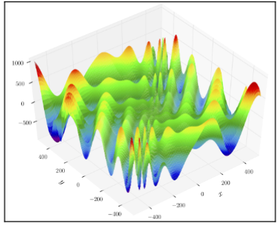
Fig. 1.5 he Eggholder function Source: https://en.wikipedia.org/wiki/File:Eggholder_function.pdf. Image by Gaortizg. Licensed under Creative Commons CC BY-SA 3.0: https://creativecommons.org/licenses/by-sa/3.0/deed.en Explore more here: https://www.sfu.ca/~ssurjano/egg.htmlhttps://www.sfu.ca/~ssurjano/egg.html#
The eggholder function is a mathematical function often used as a benchmark problem for optimization algorithms. It’s designed to be challenging due to its complex landscape with multiple local minima and one global minimum. The function is defined as:
The function has a global minimum at ( f(512, 404.2319) = -959.6407 ), which is surrounded by several local minima and maxima. The “eggholder” name comes from the visual appearance of the function’s plot, which somewhat resembles an egg holder.
Imagine you’re trying to find the lowest point on a hilly landscape, but there are many hills and valleys, and you can’t see the whole picture at once. The eggholder function is like a mathematical version of this situation. It’s used to test how well different methods, like optimization algorithms, can find the lowest point (the global minimum) in a complicated landscape with lots of ups and downs.
In high school, you might have learned about functions and how to find their minimum or maximum points. The eggholder function is special because it’s quite tricky. It has many peaks and valleys, and finding the lowest point isn’t easy. So, mathematicians and computer scientists use it to test new methods or algorithms for finding the best solution in complex situations.
1.10.2. Real Coded Operators#
1.10.2.1. Blend Crossover#
Blend Crossover. (BLX)
he α value is commonly set to 0.5, resulting in a selection interval twice as wide
as the interval between the parents.
1.10.2.2. Simulated Binary Crossover#
Simulated Binary Crossover. (SLX)
The value of β, also known as the spread factor, is calculated using a combination of a randomly chosen value and a pre-determined parameter known as η (eta), distribution index, or crowding factor. With larger values of η, offspring will tend to be more similar to their parents. Common values of η are between 10 and 20.
1.10.2.3. Normally Distributed (or Gaussian) Mutation#
Original Value is placed with a random number generated using normal distribution wit predetermined values for mean and standard deviation.
1.10.2.4. cxSimulatedBinaryBounded#
is a bounded version of cxSimulateBinary() operator, accepting the arguments low and up as the lower and upper boundaries of the search space, respectively
1.10.3. TASK: Using DEAP to calculate individual fitness using Eggholder#
When calling the implementation:
# create initial population (generation 0):
population = toolbox.populationCreator(n=POPULATION_SIZE)
# prepare the statistics object:
stats = tools.Statistics(lambda ind: ind.fitness.values)
stats.register("min", np.min)
stats.register("avg", np.mean)
# define the hall-of-fame object:
hof = tools.HallOfFame(HALL_OF_FAME_SIZE)
# perform the Genetic Algorithm flow with elitism:
population, logbook = elitism.eaSimpleWithElitism(population, toolbox, cxpb=P_CROSSOVER, mutpb=P_MUTATION,
ngen=MAX_GENERATIONS, stats=stats, halloffame=hof, verbose=True)
# print info for best solution found:
best = hof.items[0]
print("-- Best Individual = ", best)
print("-- Best Fitness = ", best.fitness.values[0])
# extract statistics:
minFitnessValues, meanFitnessValues = logbook.select("min", "avg")
# plot statistics:
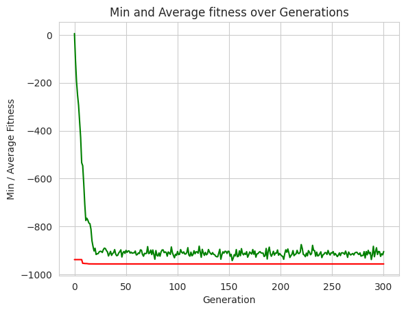
sns.set_style("whitegrid")
plt.plot(minFitnessValues, color='red')
plt.plot(meanFitnessValues, color='green')
plt.xlabel('Generation')
plt.ylabel('Min / Average Fitness')
plt.title('Min and Average fitness over Generations')
plt.show()
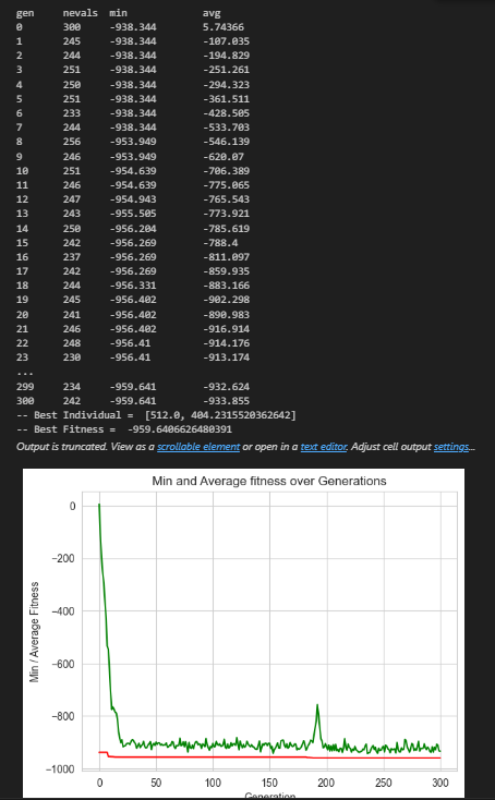
Fig. 1.6 Expected Output.#
Complete the following template:
from deap import base
from deap import creator
from deap import tools

import random
import numpy as np

import matplotlib.pyplot as plt
import seaborn as sns

import elitism

# problem constants:
DIMENSIONS = 2  # number of dimensions
BOUND_LOW, BOUND_UP = -512.0, 512.0  # boundaries for all dimensions

# Genetic Algorithm constants:
POPULATION_SIZE = 300
P_CROSSOVER = 0.9  # probability for crossover
P_MUTATION = 0.1   # (try also 0.5) probability for mutating an individual
MAX_GENERATIONS = 300
HALL_OF_FAME_SIZE = 30
CROWDING_FACTOR = 20.0  # crowding factor for crossover and mutation

# set the random seed:
RANDOM_SEED = 42
random.seed(RANDOM_SEED)

toolbox = base.Toolbox()

# TODO define a single objective, minimizing fitness strategy:


# TODO create the Individual class based on list:


# helper function for creating random real numbers uniformly distributed within a given range [low, up]
# it assumes that the range is the same for every dimension
def randomFloat(low, up):
    return [random.uniform(l, u) for l, u in zip([low] * DIMENSIONS, [up] * DIMENSIONS)]

# TODO create an operator that randomly returns a float in the desired range and dimension:


# TODO create the individual operator to fill up an Individual instance:


# TODO create the population operator to generate a list of individuals:


# TDOO Complete Eggholder function as the given individual's fitness:
def eggholder(individual):
    x = individual[0]
    y = individual[1]
    # TODO implement the Eggholder function: f(x, y) = (- (y + 47) * sin(sqrt(abs(x/2 + (y + 47)))) - x * sin(sqrt(abs(x - (y + 47))))

    return f,  # return a tuple

toolbox.register("evaluate", eggholder)

# genetic operators:
toolbox.register("select", tools.selTournament, tournsize=2)
"""
Given that the selection operator is independent5.
of the individual type, and we've had a good experience so far using the
tournament selection with a tournament size of 2, coupled with the elitist
approach, we'll continue to use it here. The crossover and mutation operators, on
the other hand, need to be specialized for floating-point numbers within given
boundaries, and therefore we use the DEAP-provided
cxSimulatedBinaryBounded operator for crossover, and
the mutPolynomialBounded operator for mutation:
"""

# TODO register the crossover operator: using 'mate' as tools.cxSimulatedBinaryBounded  and the crowding factor as CROWDING_FACTOR


# TODO register the mutation operator: using 'mutate' as tools.mutPolynomialBounded and the crowding factor as CROWDING_FACTOR
from deap import base
from deap import creator
from deap import tools

import random
import numpy as np

import matplotlib.pyplot as plt
import seaborn as sns

import elitism

# problem constants:
DIMENSIONS = 2  # number of dimensions
BOUND_LOW, BOUND_UP = -512.0, 512.0  # boundaries for all dimensions

# Genetic Algorithm constants:
POPULATION_SIZE = 300
P_CROSSOVER = 0.9  # probability for crossover
P_MUTATION = 0.1   # (try also 0.5) probability for mutating an individual
MAX_GENERATIONS = 300
HALL_OF_FAME_SIZE = 30
CROWDING_FACTOR = 20.0  # crowding factor for crossover and mutation

# set the random seed:
RANDOM_SEED = 42
random.seed(RANDOM_SEED)

toolbox = base.Toolbox()

# define a single objective, minimizing fitness strategy:
creator.create("FitnessMin", base.Fitness, weights=(-1.0,))

# create the Individual class based on list:
creator.create("Individual", list, fitness=creator.FitnessMin)


# helper function for creating random real numbers uniformly distributed within a given range [low, up]
# it assumes that the range is the same for every dimension
def randomFloat(low, up):
    return [random.uniform(l, u) for l, u in zip([low] * DIMENSIONS, [up] * DIMENSIONS)]

# create an operator that randomly returns a float in the desired range and dimension:
toolbox.register("attrFloat", randomFloat, BOUND_LOW, BOUND_UP)

# create the individual operator to fill up an Individual instance:
toolbox.register("individualCreator", tools.initIterate, creator.Individual, toolbox.attrFloat)

# create the population operator to generate a list of individuals:
toolbox.register("populationCreator", tools.initRepeat, list, toolbox.individualCreator)


# Eggholder function as the given individual's fitness:
def eggholder(individual):
    x = individual[0]
    y = individual[1]
    f = (-(y + 47.0) * np.sin(np.sqrt(abs(x/2.0 + (y + 47.0)))) - x * np.sin(np.sqrt(abs(x - (y + 47.0)))))
    return f,  # return a tuple

toolbox.register("evaluate", eggholder)

# genetic operators:
toolbox.register("select", tools.selTournament, tournsize=2)
toolbox.register("mate", tools.cxSimulatedBinaryBounded, low=BOUND_LOW, up=BOUND_UP, eta=CROWDING_FACTOR)
toolbox.register("mutate", tools.mutPolynomialBounded, low=BOUND_LOW, up=BOUND_UP, eta=CROWDING_FACTOR, indpb=1.0/DIMENSIONS)
# create initial population (generation 0):
population = toolbox.populationCreator(n=POPULATION_SIZE)

# prepare the statistics object:
stats = tools.Statistics(lambda ind: ind.fitness.values)
stats.register("min", np.min)
stats.register("avg", np.mean)

# define the hall-of-fame object:
hof = tools.HallOfFame(HALL_OF_FAME_SIZE)

# perform the Genetic Algorithm flow with elitism:
population, logbook = elitism.eaSimpleWithElitism(population, toolbox, cxpb=P_CROSSOVER, mutpb=P_MUTATION,
                                            ngen=MAX_GENERATIONS, stats=stats, halloffame=hof, verbose=True)

# print info for best solution found:
best = hof.items[0]
print("-- Best Individual = ", best)
print("-- Best Fitness = ", best.fitness.values[0])

# extract statistics:
minFitnessValues, meanFitnessValues = logbook.select("min", "avg")

# plot statistics:
sns.set_style("whitegrid")
plt.plot(minFitnessValues, color='red')
plt.plot(meanFitnessValues, color='green')
plt.xlabel('Generation')
plt.ylabel('Min / Average Fitness')
plt.title('Min and Average fitness over Generations')

plt.show()
gen	nevals	min     	avg
0  	300   	-938.344	5.74366
1  	245   	-938.344	-107.035
2  	244   	-938.344	-194.829
3  	251   	-938.344	-251.261
4  	250   	-938.344	-294.323
5  	251   	-938.344	-361.511
6  	233   	-938.344	-428.505
7  	244   	-938.344	-533.703
8  	256   	-953.949	-546.139
9  	246   	-953.949	-620.07
10 	251   	-954.639	-706.389
11 	246   	-954.639	-775.065
12 	247   	-954.943	-765.543
13 	243   	-955.505	-773.921
14 	250   	-956.204	-785.619
15 	242   	-956.269	-788.4
16 	237   	-956.269	-811.097
17 	242   	-956.269	-859.935
18 	244   	-956.331	-883.166
19 	245   	-956.402	-902.298
20 	241   	-956.402	-890.983
21 	246   	-956.402	-916.914
22 	248   	-956.41 	-914.176
23 	230   	-956.41 	-913.174
24 	258   	-956.41 	-905.963
25 	240   	-956.415	-903.579
26 	253   	-956.416	-904.171
27 	247   	-956.416	-908.573
28 	262   	-956.416	-896.797
29 	249   	-956.416	-890.515
30 	249   	-956.416	-892.158
31 	248   	-956.418	-900.733
32 	241   	-956.418	-905.919
33 	251   	-956.418	-923.118
34 	254   	-956.419	-913.551
35 	243   	-956.419	-903.915
36 	254   	-956.419	-920.719
37 	244   	-956.419	-913.107
38 	246   	-956.419	-909.078
39 	237   	-956.419	-896.549
40 	249   	-956.419	-915.218
41 	244   	-956.419	-922.198
42 	242   	-956.419	-920.011
43 	242   	-956.419	-910.241
44 	256   	-956.419	-904.912
45 	250   	-956.419	-897.528
46 	250   	-956.419	-927.587
47 	243   	-956.419	-910.139
48 	254   	-956.419	-904.402
49 	256   	-956.419	-912.471
50 	244   	-956.419	-899.757
51 	243   	-956.421	-907.919
52 	235   	-956.421	-902.346
53 	252   	-956.421	-902.17
54 	247   	-956.421	-911.081
55 	228   	-956.421	-907.036
56 	243   	-956.421	-911.801
57 	249   	-956.421	-909.967
58 	232   	-956.421	-910.203
59 	254   	-956.422	-902.523
60 	248   	-956.422	-918.906
61 	246   	-956.422	-917.013
62 	242   	-956.422	-910.31
63 	240   	-956.422	-912.768
64 	251   	-956.422	-897.512
65 	249   	-956.422	-899.223
66 	255   	-956.422	-916.923
67 	241   	-956.422	-924.08
68 	254   	-956.422	-912.092
69 	246   	-956.422	-913.548
70 	255   	-956.422	-911.423
71 	248   	-956.422	-884.076
72 	248   	-956.422	-913.138
73 	246   	-956.422	-910.744
74 	252   	-956.423	-898.459
75 	245   	-956.423	-917.205
76 	247   	-956.423	-898.008
77 	248   	-956.423	-916.493
78 	250   	-956.423	-936.691
79 	250   	-956.423	-900.525
80 	250   	-956.423	-920.197
81 	244   	-956.423	-923.536
82 	253   	-956.423	-910.414
83 	259   	-956.423	-924.097
84 	246   	-956.423	-906.337
85 	256   	-956.424	-898.217
86 	250   	-956.424	-897.675
87 	244   	-956.424	-909.308
88 	255   	-956.424	-906.221
89 	234   	-956.424	-908.244
90 	254   	-956.424	-923.972
91 	249   	-956.424	-906.336
92 	257   	-956.424	-911.165
93 	251   	-956.424	-916.505
94 	244   	-956.424	-885.511
95 	233   	-956.424	-908.822
96 	246   	-956.424	-920.647
97 	249   	-956.424	-930.739
98 	252   	-956.424	-915.898
99 	235   	-956.424	-920.517
100	251   	-956.424	-904.436
101	241   	-956.424	-917.366
102	256   	-956.424	-915.778
103	246   	-956.424	-896.39
104	254   	-956.424	-907.495
105	240   	-956.424	-911.764
106	252   	-956.424	-906.007
107	254   	-956.424	-915.019
108	232   	-956.424	-914.954
109	256   	-956.424	-908.935
110	235   	-956.424	-888.409
111	239   	-956.424	-919.367
112	262   	-956.424	-923.914
113	250   	-956.424	-907.117
114	233   	-956.424	-922.384
115	249   	-956.424	-917.331
116	243   	-956.424	-901.383
117	245   	-956.424	-913.967
118	247   	-956.424	-905.714
119	243   	-956.424	-906.011
120	256   	-956.424	-911.673
121	247   	-956.424	-882.289
122	238   	-956.424	-907.098
123	233   	-956.424	-928.467
124	237   	-956.424	-895.269
125	250   	-956.424	-910.376
126	246   	-956.424	-920.847
127	232   	-956.424	-908.048
128	229   	-956.424	-918.347
129	239   	-956.424	-914.269
130	234   	-956.424	-896.169
131	246   	-956.424	-906.654
132	244   	-956.424	-912.741
133	247   	-956.424	-916.772
134	240   	-956.424	-909.066
135	240   	-956.424	-916.434
136	250   	-956.424	-917.727
137	242   	-956.424	-924.111
138	251   	-956.424	-926.445
139	241   	-956.424	-926.225
140	244   	-956.424	-910.779
141	239   	-956.424	-895.076
142	249   	-956.424	-936.617
143	243   	-956.424	-918.654
144	246   	-956.424	-905.852
145	241   	-956.424	-911.301
146	253   	-956.424	-903.52
147	238   	-956.424	-904.164
148	251   	-956.424	-912.806
149	250   	-956.424	-903.45
150	253   	-956.424	-904.088
151	239   	-956.424	-924.06
152	249   	-956.424	-916.081
153	243   	-956.424	-942.513
154	248   	-956.424	-932.63
155	246   	-956.424	-917.954
156	244   	-956.424	-922.958
157	246   	-956.424	-896.53
158	234   	-956.424	-926.204
159	239   	-956.424	-924.613
160	245   	-956.424	-901.713
161	245   	-956.424	-922.182
162	255   	-956.426	-892.473
163	242   	-956.426	-912.645
164	238   	-956.426	-918.48
165	248   	-956.427	-911.584
166	239   	-956.427	-916.627
167	250   	-956.428	-905.225
168	247   	-956.428	-928.306
169	232   	-956.428	-918.574
170	244   	-956.428	-906.343
171	241   	-956.428	-911.253
172	249   	-956.428	-915.307
173	253   	-956.428	-896.207
174	246   	-956.428	-915.972
175	238   	-956.428	-902.406
176	239   	-956.428	-928.118
177	250   	-956.428	-914.629
178	249   	-956.428	-913.461
179	253   	-956.428	-907.954
180	248   	-956.428	-905.022
181	253   	-956.428	-910.216
182	231   	-956.428	-911.189
183	243   	-956.43 	-911.191
184	242   	-956.43 	-925.442
185	244   	-956.431	-921.63
186	245   	-956.432	-891.744
187	258   	-956.432	-935.833
188	260   	-956.433	-903.166
189	250   	-956.433	-886.175
190	224   	-956.434	-913.754
191	240   	-956.434	-924.412
192	231   	-956.436	-915.58
193	239   	-956.436	-903.564
194	249   	-956.436	-919.602
195	256   	-956.436	-910.832
196	241   	-956.436	-911.517
197	254   	-956.436	-897.949
198	245   	-956.436	-920.07
199	254   	-956.436	-912.692
200	239   	-956.436	-917.938
201	251   	-956.437	-922.538
202	231   	-956.437	-924.769
203	250   	-956.437	-937.061
204	243   	-956.437	-913.575
205	251   	-956.437	-897.464
206	245   	-956.437	-907.549
207	243   	-956.438	-893.863
208	248   	-956.438	-910.494
209	244   	-956.438	-929.546
210	243   	-956.438	-921.691
211	244   	-956.438	-915.993
212	246   	-956.438	-900.64
213	245   	-956.438	-922.004
214	245   	-956.438	-917.053
215	244   	-956.438	-914.101
216	232   	-956.438	-899.716
217	251   	-956.438	-912.403
218	241   	-956.438	-912.709
219	247   	-956.438	-907.405
220	257   	-956.438	-875.374
221	243   	-956.438	-891.936
222	250   	-956.438	-916.659
223	221   	-956.438	-918.934
224	244   	-956.438	-926.057
225	245   	-956.438	-911.212
226	248   	-956.438	-922.454
227	237   	-956.438	-900.819
228	231   	-956.438	-907.826
229	243   	-956.438	-918.015
230	252   	-956.438	-913.237
231	237   	-956.438	-878.731
232	251   	-956.438	-900.097
233	248   	-956.438	-900.924
234	254   	-956.438	-924.308
235	245   	-956.438	-906.918
236	245   	-956.438	-923.083
237	251   	-956.438	-921.034
238	238   	-956.438	-913.661
239	246   	-956.438	-905.738
240	245   	-956.438	-929.993
241	253   	-956.438	-919.128
242	256   	-956.439	-915.749
243	249   	-956.439	-909.29
244	243   	-956.439	-909.373
245	235   	-956.439	-916.971
246	233   	-956.439	-900.165
247	243   	-956.457	-912.683
248	243   	-956.457	-919.149
249	250   	-956.457	-909.71
250	241   	-956.457	-910.937
251	245   	-956.457	-904.929
252	248   	-956.457	-919.619
253	247   	-956.457	-912.736
254	234   	-956.457	-918.784
255	244   	-956.459	-925.623
256	237   	-956.459	-919.741
257	236   	-956.459	-910.309
258	248   	-956.461	-921.644
259	248   	-956.461	-910.286
260	242   	-956.462	-909.81
261	236   	-956.462	-911.066
262	243   	-956.462	-916.376
263	245   	-956.462	-902.628
264	247   	-956.462	-913.946
265	243   	-956.462	-929.052
266	245   	-956.462	-906.68
267	251   	-956.462	-914.606
268	246   	-956.462	-919.04
269	246   	-956.462	-915.43
270	248   	-956.462	-912.863
271	252   	-956.464	-918.89
272	241   	-956.464	-910.356
273	248   	-956.464	-908.291
274	244   	-956.464	-907.585
275	242   	-956.464	-913.868
276	251   	-956.464	-917.028
277	236   	-956.464	-910.128
278	245   	-956.464	-923.969
279	244   	-956.464	-921.06
280	250   	-956.464	-921.351
281	253   	-956.464	-904.838
282	248   	-956.464	-931.469
283	244   	-956.464	-904.758
284	253   	-956.464	-918.484
285	253   	-956.464	-899.707
286	249   	-956.464	-913.501
287	242   	-956.464	-908.205
288	248   	-956.464	-938.159
289	249   	-956.464	-918.186
290	246   	-956.464	-882.741
291	251   	-956.464	-926.314
292	244   	-956.464	-905.242
293	245   	-956.464	-888.759
294	249   	-956.464	-917.127
295	243   	-956.464	-904.123
296	243   	-956.464	-905.527
297	250   	-956.464	-924.859
298	244   	-956.464	-913.924
299	242   	-956.464	-918.374
300	245   	-956.464	-904.471
-- Best Individual =  [483.909780775573, 434.4287397072944]
-- Best Fitness =  -956.4641087935356
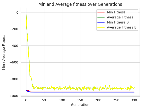
1.10.4. TASK Replot with 0.5 Mutation and show on the same plot#
from deap import base
from deap import creator
from deap import tools

import random
import numpy as np

import matplotlib.pyplot as plt
import seaborn as sns

import elitism

# problem constants:
DIMENSIONS = 2  # number of dimensions
BOUND_LOW, BOUND_UP = -512.0, 512.0  # boundaries for all dimensions

# Genetic Algorithm constants:
POPULATION_SIZE = 300
P_CROSSOVER = 0.9  # probability for crossover
P_MUTATION = 0.5   # (try also 0.5) probability for mutating an individual
MAX_GENERATIONS = 300
HALL_OF_FAME_SIZE = 30
CROWDING_FACTOR = 20.0  # crowding factor for crossover and mutation

# set the random seed:
RANDOM_SEED = 42
random.seed(RANDOM_SEED)

toolbox = base.Toolbox()

# define a single objective, minimizing fitness strategy:
creator.create("FitnessMin", base.Fitness, weights=(-1.0,))

# create the Individual class based on list:
creator.create("Individual", list, fitness=creator.FitnessMin)


# helper function for creating random real numbers uniformly distributed within a given range [low, up]
# it assumes that the range is the same for every dimension
def randomFloat(low, up):
    return [random.uniform(l, u) for l, u in zip([low] * DIMENSIONS, [up] * DIMENSIONS)]

# create an operator that randomly returns a float in the desired range and dimension:
toolbox.register("attrFloat", randomFloat, BOUND_LOW, BOUND_UP)

# create the individual operator to fill up an Individual instance:
toolbox.register("individualCreator", tools.initIterate, creator.Individual, toolbox.attrFloat)

# create the population operator to generate a list of individuals:
toolbox.register("populationCreator", tools.initRepeat, list, toolbox.individualCreator)


# Eggholder function as the given individual's fitness:
def eggholder(individual):
    x = individual[0]
    y = individual[1]
    f = (-(y + 47.0) * np.sin(np.sqrt(abs(x/2.0 + (y + 47.0)))) - x * np.sin(np.sqrt(abs(x - (y + 47.0)))))
    return f,  # return a tuple

toolbox.register("evaluate", eggholder)

# genetic operators:
toolbox.register("select", tools.selTournament, tournsize=2)
toolbox.register("mate", tools.cxSimulatedBinaryBounded, low=BOUND_LOW, up=BOUND_UP, eta=CROWDING_FACTOR)
toolbox.register("mutate", tools.mutPolynomialBounded, low=BOUND_LOW, up=BOUND_UP, eta=CROWDING_FACTOR, indpb=1.0/DIMENSIONS)
# TODO Show in sam eplot but as blue and yellow lines instead. with the previous plot

# create initial population (generation 0):
population_b = toolbox.populationCreator(n=POPULATION_SIZE)

# prepare the statistics object:
stats_b = tools.Statistics(lambda ind: ind.fitness.values)
stats_b.register("min", np.min)
stats_b.register("avg", np.mean)

# define the hall-of-fame object:
hof = tools.HallOfFame(HALL_OF_FAME_SIZE)

# perform the Genetic Algorithm flow with elitism:
population_b, logbook_b = elitism.eaSimpleWithElitism(population_b, toolbox, cxpb=P_CROSSOVER, mutpb=P_MUTATION,
                                            ngen=MAX_GENERATIONS, stats=stats_b, halloffame=hof, verbose=True)

# print info for best solution found:
best = hof.items[0]
print("-- Best Individual = ", best)
print("-- Best Fitness = ", best.fitness.values[0])

# extract statistics:
minFitnessValues_b, meanFitnessValues_b = logbook_b.select("min", "avg")

# plot statistics:
sns.set_style("whitegrid")
plt.plot(minFitnessValues, color='red')
plt.plot(meanFitnessValues, color='green')
plt.plot(minFitnessValues_b, color='blue')
plt.plot(meanFitnessValues, color='yellow')

plt.xlabel('Generation')
plt.ylabel('Min / Average Fitness')

# Add legends.
plt.legend(['Min Fitness', 'Average Fitness', 'Min Fitness B', 'Average Fitness B'])

plt.title('Min and Average fitness over Generations')


plt.show()
gen	nevals	min     	avg
0  	300   	-938.344	5.74366
1  	256   	-938.344	-93.6859
2  	261   	-938.344	-199.776
3  	260   	-938.344	-242.383
4  	257   	-949.799	-277.752
5  	255   	-949.799	-340.727
6  	255   	-951.464	-401.777
7  	258   	-951.464	-458.552
8  	254   	-951.464	-464.904
9  	258   	-952.016	-540.356
10 	249   	-954.245	-569.033
11 	254   	-958.514	-548.672
12 	261   	-958.514	-577.511
13 	254   	-959.024	-578.77
14 	248   	-959.024	-595.563
15 	261   	-959.285	-587.904
16 	256   	-959.304	-618.27
17 	259   	-959.377	-596.288
18 	256   	-959.485	-638.201
19 	262   	-959.508	-670.193
20 	253   	-959.557	-705.507
21 	260   	-959.575	-702.257
22 	256   	-959.606	-716.336
23 	264   	-959.636	-715.322
24 	256   	-959.636	-771.18
25 	263   	-959.636	-763.546
26 	262   	-959.638	-739.197
27 	255   	-959.638	-751.84
28 	265   	-959.638	-795.878
29 	256   	-959.638	-752.338
30 	256   	-959.639	-757.67
31 	251   	-959.64 	-762.326
32 	252   	-959.64 	-734.005
33 	258   	-959.64 	-758.626
34 	250   	-959.64 	-731.062
35 	250   	-959.64 	-717.838
36 	251   	-959.64 	-745.382
37 	259   	-959.641	-753.785
38 	255   	-959.641	-741.456
39 	261   	-959.641	-721.202
40 	262   	-959.641	-739.42
41 	259   	-959.641	-780.229
42 	255   	-959.641	-734.662
43 	250   	-959.641	-747.223
44 	255   	-959.641	-756.578
45 	257   	-959.641	-720.683
46 	254   	-959.641	-794.43
47 	254   	-959.641	-753.234
48 	250   	-959.641	-745.042
49 	261   	-959.641	-726.402
50 	261   	-959.641	-736.484
51 	263   	-959.641	-714.715
52 	255   	-959.641	-751.426
53 	255   	-959.641	-762.815
54 	254   	-959.641	-766.396
55 	260   	-959.641	-738.426
56 	263   	-959.641	-752.669
57 	256   	-959.641	-745.656
58 	262   	-959.641	-777.061
59 	254   	-959.641	-750.837
60 	254   	-959.641	-752.566
61 	266   	-959.641	-765.31
62 	252   	-959.641	-738.543
63 	264   	-959.641	-728.439
64 	263   	-959.641	-742.71
65 	262   	-959.641	-725.614
66 	260   	-959.641	-714.957
67 	258   	-959.641	-699.017
68 	255   	-959.641	-762.248
69 	259   	-959.641	-753.336
70 	258   	-959.641	-724.914
71 	259   	-959.641	-756.512
72 	258   	-959.641	-746.023
73 	247   	-959.641	-797.67
74 	252   	-959.641	-789.766
75 	262   	-959.641	-776.967
76 	257   	-959.641	-780.892
77 	257   	-959.641	-760.575
78 	257   	-959.641	-744.508
79 	261   	-959.641	-766.537
80 	260   	-959.641	-758.173
81 	255   	-959.641	-737.503
82 	257   	-959.641	-740.326
83 	258   	-959.641	-775.877
84 	257   	-959.641	-751.299
85 	258   	-959.641	-749.458
86 	256   	-959.641	-720.814
87 	254   	-959.641	-709.52
88 	255   	-959.641	-686.135
89 	258   	-959.641	-738.067
90 	243   	-959.641	-774.626
91 	258   	-959.641	-755.753
92 	257   	-959.641	-741.26
93 	255   	-959.641	-760.156
94 	254   	-959.641	-708.15
95 	252   	-959.641	-744.25
96 	252   	-959.641	-767.987
97 	254   	-959.641	-776.67
98 	252   	-959.641	-785.319
99 	263   	-959.641	-755.387
100	258   	-959.641	-737.3
101	254   	-959.641	-746.734
102	253   	-959.641	-727.907
103	248   	-959.641	-733.329
104	246   	-959.641	-724.901
105	259   	-959.641	-758.727
106	256   	-959.641	-749.133
107	250   	-959.641	-763.872
108	253   	-959.641	-737.578
109	260   	-959.641	-715.57
110	259   	-959.641	-749.636
111	259   	-959.641	-750.613
112	262   	-959.641	-744.497
113	267   	-959.641	-730.266
114	259   	-959.641	-800.164
115	258   	-959.641	-784.857
116	247   	-959.641	-742.412
117	261   	-959.641	-794.012
118	262   	-959.641	-768.131
119	257   	-959.641	-772.022
120	259   	-959.641	-730.852
121	245   	-959.641	-739.778
122	258   	-959.641	-740.574
123	256   	-959.641	-701.608
124	257   	-959.641	-755.13
125	255   	-959.641	-759.577
126	255   	-959.641	-804.498
127	262   	-959.641	-739.028
128	257   	-959.641	-763.068
129	262   	-959.641	-744.232
130	258   	-959.641	-748.839
131	260   	-959.641	-764.929
132	244   	-959.641	-783.832
133	262   	-959.641	-732.722
134	253   	-959.641	-733.872
135	253   	-959.641	-719.554
136	250   	-959.641	-748.439
137	256   	-959.641	-766.022
138	249   	-959.641	-759.738
139	253   	-959.641	-763.703
140	254   	-959.641	-726.936
141	257   	-959.641	-709.665
142	256   	-959.641	-736.185
143	260   	-959.641	-762.962
144	246   	-959.641	-789.74
145	245   	-959.641	-731.139
146	258   	-959.641	-742.358
147	252   	-959.641	-779.884
148	257   	-959.641	-752.867
149	260   	-959.641	-752.175
150	255   	-959.641	-725.182
151	263   	-959.641	-777.36
152	263   	-959.641	-770.311
153	261   	-959.641	-762.673
154	256   	-959.641	-746.876
155	257   	-959.641	-739.719
156	259   	-959.641	-744.049
157	263   	-959.641	-751.625
158	258   	-959.641	-768.99
159	261   	-959.641	-723.516
160	262   	-959.641	-713.253
161	263   	-959.641	-748.435
162	259   	-959.641	-748.054
163	255   	-959.641	-773.437
164	258   	-959.641	-746.575
165	258   	-959.641	-737.424
166	262   	-959.641	-769.593
167	256   	-959.641	-735.236
168	253   	-959.641	-721.385
169	251   	-959.641	-761.908
170	254   	-959.641	-789.053
171	264   	-959.641	-755.806
172	248   	-959.641	-730.442
173	255   	-959.641	-750.957
174	258   	-959.641	-780.144
175	257   	-959.641	-755.878
176	255   	-959.641	-766.571
177	261   	-959.641	-743.843
178	254   	-959.641	-747.481
179	257   	-959.641	-742.401
180	262   	-959.641	-739.047
181	258   	-959.641	-697.684
182	263   	-959.641	-797.708
183	263   	-959.641	-769.063
184	259   	-959.641	-738.333
185	255   	-959.641	-753.46
186	261   	-959.641	-745.397
187	241   	-959.641	-729.586
188	252   	-959.641	-756.608
189	258   	-959.641	-723.37
190	254   	-959.641	-724.19
191	260   	-959.641	-763.635
192	260   	-959.641	-769.969
193	257   	-959.641	-748.303
194	251   	-959.641	-751.2
195	261   	-959.641	-725.999
196	256   	-959.641	-755.321
197	254   	-959.641	-747.918
198	256   	-959.641	-718.149
199	253   	-959.641	-745.203
200	250   	-959.641	-747.445
201	260   	-959.641	-779.561
202	258   	-959.641	-776.306
203	248   	-959.641	-753.287
204	261   	-959.641	-752.361
205	254   	-959.641	-733.352
206	253   	-959.641	-741.351
207	251   	-959.641	-726.527
208	253   	-959.641	-729.826
209	254   	-959.641	-733.898
210	250   	-959.641	-750.296
211	257   	-959.641	-758.197
212	260   	-959.641	-777.239
213	259   	-959.641	-685.463
214	257   	-959.641	-716.25
215	257   	-959.641	-721.161
216	251   	-959.641	-763.303
217	250   	-959.641	-777.05
218	261   	-959.641	-755.264
219	249   	-959.641	-763.745
220	250   	-959.641	-753.404
221	257   	-959.641	-753.239
222	260   	-959.641	-734.601
223	257   	-959.641	-734.809
224	249   	-959.641	-740.223
225	252   	-959.641	-731.885
226	246   	-959.641	-768.486
227	248   	-959.641	-732.126
228	254   	-959.641	-748.677
229	267   	-959.641	-756.971
230	259   	-959.641	-710.17
231	257   	-959.641	-752.838
232	254   	-959.641	-746.258
233	262   	-959.641	-732.468
234	257   	-959.641	-721.263
235	253   	-959.641	-747.722
236	261   	-959.641	-770.98
237	260   	-959.641	-757.523
238	256   	-959.641	-728.39
239	252   	-959.641	-771.427
240	259   	-959.641	-755.311
241	260   	-959.641	-757.264
242	262   	-959.641	-780.184
243	259   	-959.641	-733.485
244	261   	-959.641	-735.899
245	256   	-959.641	-730.978
246	258   	-959.641	-787.235
247	254   	-959.641	-754.902
248	257   	-959.641	-770.294
249	266   	-959.641	-772.589
250	257   	-959.641	-754.046
251	254   	-959.641	-727.615
252	263   	-959.641	-753.933
253	256   	-959.641	-766.426
254	253   	-959.641	-734.06
255	252   	-959.641	-732.101
256	248   	-959.641	-787.523
257	257   	-959.641	-759.938
258	260   	-959.641	-767.575
259	257   	-959.641	-729.381
260	257   	-959.641	-722.87
261	249   	-959.641	-783.715
262	246   	-959.641	-755.976
263	263   	-959.641	-752.765
264	258   	-959.641	-760.53
265	258   	-959.641	-725.087
266	246   	-959.641	-749.353
267	259   	-959.641	-748.779
268	257   	-959.641	-687.252
269	254   	-959.641	-705.406
270	248   	-959.641	-761.802
271	252   	-959.641	-753.18
272	259   	-959.641	-773.835
273	262   	-959.641	-722.396
274	258   	-959.641	-747.301
275	260   	-959.641	-732.403
276	256   	-959.641	-763.088
277	250   	-959.641	-749.093
278	250   	-959.641	-757.96
279	247   	-959.641	-766.822
280	253   	-959.641	-767.009
281	258   	-959.641	-738.958
282	257   	-959.641	-769.827
283	256   	-959.641	-777.053
284	254   	-959.641	-756.768
285	260   	-959.641	-736.25
286	254   	-959.641	-755.565
287	257   	-959.641	-774.093
288	255   	-959.641	-744.925
289	247   	-959.641	-789.205
290	259   	-959.641	-746.968
291	251   	-959.641	-710.721
292	250   	-959.641	-715.619
293	252   	-959.641	-704.073
294	259   	-959.641	-707.549
295	249   	-959.641	-750.2
296	252   	-959.641	-764.914
297	254   	-959.641	-777.263
298	257   	-959.641	-774.444
299	257   	-959.641	-780.336
300	256   	-959.641	-778.702
-- Best Individual =  [512.0, 404.2318049696766]
-- Best Fitness =  -959.640662720851