1.4. The Traveling Salesman#
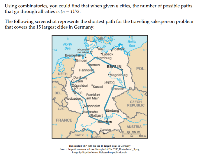
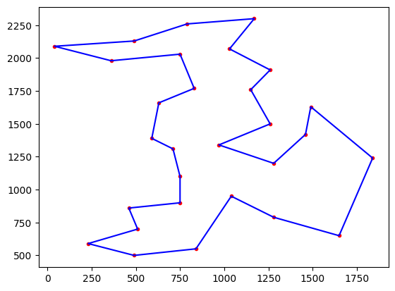
“Given a list of cities and the distances between each pair of the cities, find the shortest possible path that goes through all the cities, and returns to the starting city.”
1.4.1. Resources#
1.4.2. Activity Building the Traveling Salesman Problem#
1.4.2.1. Problem#
Note
Create a class named
TravelingSalesmanProblemthat will have the following methods:def __init__(self, name):Creates Instancesdef __len__(self):Returns the length of the number of cities.def __createData(self):Creates the data from the file.def getTotalDistance(self, indices):Returns the total distance of the path.def plotData(self, indices):Plots the data.
Test it with the following:
tsp = TravelingSalesmanProblem("bayg29")
# generate a random solution and evaluate it:
#randomSolution = random.sample(range(len(tsp)), len(tsp))
# see http://elib.zib.de/pub/mp-testdata/tsp/tsplib/tsp/bayg29.opt.tour
optimalSolution = [0, 27, 5, 11, 8, 25, 2, 28, 4, 20, 1, 19, 9, 3, 14, 17, 13, 16, 21, 10, 18, 24, 6, 22, 7, 26, 15, 12, 23]
print("Problem name: " + tsp.name)
print("Optimal solution = ", optimalSolution)
print("Optimal distance = ", tsp.getTotalDistance(optimalSolution))
# plot the solution:
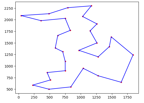
plot = tsp.plotData(optimalSolution)
plot.show()
It should print the following:
Problem name: bayg29
Optimal solution =  [0, 27, 5, 11, 8, 25, 2, 28, 4, 20, 1, 19, 9, 3, 14, 17, 13, 16, 21, 10, 18, 24, 6, 22, 7, 26, 15, 12, 23]
Optimal distance =  9074.147
1.4.2.2. Solution#
import csv
import pickle
import os
import codecs

import numpy as np

from urllib.request import urlopen

import matplotlib.pyplot as plt
class TravelingSalesmanProblem:
    """This class encapsulates the Traveling Salesman Problem.
    City coordinates are read from an online file and distance matrix is calculated.
    The data is serialized to disk.
    The total distance can be calculated for a path represented by a list of city indices.
    A plot can be created for a path represented by a list of city indices.

    :param name: The name of the corresponding TSPLIB problem, e.g. 'burma14' or 'bayg29'.
    """

    def __init__(self, name):
        """
        Creates an instance of a TSP

        :param name: name of the TSP problem
        """

        # initialize instance variables:
        self.name = name
        self.locations = []
        self.distances = []
        self.tspSize = 0

        # initialize the data:
        self.__initData()

    def __len__(self):
        """
        returns the length of the underlying TSP
        :return: the length of the underlying TSP (number of cities)
        """
        return self.tspSize

    def __initData(self):
        """Reads the serialized data, and if not available - calls __create_data() to prepare it
        """

        # attempt to read serialized data:
        try:
            self.locations = pickle.load(open(os.path.join("tsp-data", self.name + "-loc.pickle"), "rb"))
            self.distances = pickle.load(open(os.path.join("tsp-data", self.name + "-dist.pickle"), "rb"))
        except (OSError, IOError):
            pass

        # serailized data not found - create the data from scratch:
        if not self.locations or not self.distances:
            self.__createData()

        # set the problem 'size':
        self.tspSize = len(self.locations)

    def __createData(self):
        """Reads the desired TSP file from the Internet, extracts the city coordinates, calculates the distances
        between every two cities and uses them to populate a distance matrix (two-dimensional array).
        It then serializes the city locations and the calculated distances to disk using the pickle utility.
        """
        self.locations = []

        # print("http://elib.zib.de/pub/mp-testdata/tsp/tsplib/tsp/" + self.name + ".tsp")

        # Use the following instead: https://raw.githubusercontent.com/mastqe/tsplib/master/a280.tsp
        URL = "https://raw.githubusercontent.com/mastqe/tsplib/master/"
        print(URL + self.name + ".tsp")
        # open whitespace-delimited file from url and read lines from it:
        with urlopen(URL + self.name + ".tsp") as f:
            reader = csv.reader(codecs.iterdecode(f, 'utf-8'), delimiter=" ", skipinitialspace=True)

            # skip lines until one of these lines is found:
            for row in reader:
                if row[0] in ('DISPLAY_DATA_SECTION', 'NODE_COORD_SECTION'):
                    break

            # read data lines until 'EOF' found:
            for row in reader:
                if row[0] != 'EOF':
                    # remove index at beginning of line:
                    del row[0]

                    # convert x,y coordinates to ndarray:
                    self.locations.append(np.asarray(row, dtype=np.float32))
                else:
                    break

            # set the problem 'size':
            self.tspSize = len(self.locations)

            # print data:
            print("length = {}, locations = {}".format(self.tspSize, self.locations))

            # initialize distance matrix by filling it with 0's:
            self.distances = [[0] * self.tspSize for _ in range(self.tspSize)]

            # populate the distance matrix with calculated distances:
            for i in range(self.tspSize):
                for j in range(i + 1, self.tspSize):
                    # calculate euclidean distance between two ndarrays:
                    distance = np.linalg.norm(self.locations[j] - self.locations[i])
                    self.distances[i][j] = distance
                    self.distances[j][i] = distance
                    print("{}, {}: location1 = {}, location2 = {} => distance = {}".format(i, j, self.locations[i], self.locations[j], distance))

            # serialize locations and distances:
            if not os.path.exists("tsp-data"):
                os.makedirs("tsp-data")
            pickle.dump(self.locations, open(os.path.join("tsp-data", self.name + "-loc.pickle"), "wb"))
            pickle.dump(self.distances, open(os.path.join("tsp-data", self.name + "-dist.pickle"), "wb"))

    def getTotalDistance(self, indices):
        """Calculates the total distance of the path described by the given indices of the cities

        :param indices: A list of ordered city indices describing the given path.
        :return: total distance of the path described by the given indices
        """
        # distance between th elast and first city:
        distance = self.distances[indices[-1]][indices[0]]

        # add the distance between each pair of consequtive cities:
        for i in range(len(indices) - 1):
            distance += self.distances[indices[i]][indices[i + 1]]

        return distance

    def plotData(self, indices):
        """plots the path described by the given indices of the cities

        :param indices: A list of ordered city indices describing the given path.
        :return: the resulting plot
        """

        # plot the dots representing the cities:
        plt.scatter(*zip(*self.locations), marker='.', color='red')

        # create a list of the corresponding city locations:
        locs = [self.locations[i] for i in indices]
        locs.append(locs[0])

        # plot a line between each pair of consequtive cities:
        plt.plot(*zip(*locs), linestyle='-', color='blue')

        return plt
tsp = TravelingSalesmanProblem("bayg29")

# generate a random solution and evaluate it:
#randomSolution = random.sample(range(len(tsp)), len(tsp))

# see http://elib.zib.de/pub/mp-testdata/tsp/tsplib/tsp/bayg29.opt.tour
optimalSolution = [0, 27, 5, 11, 8, 25, 2, 28, 4, 20, 1, 19, 9, 3, 14, 17, 13, 16, 21, 10, 18, 24, 6, 22, 7, 26, 15, 12, 23]

print("Problem name: " + tsp.name)
print("Optimal solution = ", optimalSolution)
print("Optimal distance = ", tsp.getTotalDistance(optimalSolution))

# plot the solution:
plot = tsp.plotData(optimalSolution)
plot.show()
Problem name: bayg29
Optimal solution =  [0, 27, 5, 11, 8, 25, 2, 28, 4, 20, 1, 19, 9, 3, 14, 17, 13, 16, 21, 10, 18, 24, 6, 22, 7, 26, 15, 12, 23]
Optimal distance =  9074.147
1.4.3. Solving TSP Using DEAP Framework#
1.4.3.1. Problem#
Now you will use the Deap framework to evaluate and find the best solutions. Use the following parameters:
POPULATION SIZE = 300
NUMBER OF GENERATIONS = 100
HALL_OF_FAME_SIZE = 1
Probability of crossover = 0.9
Probability of mutation = 0.1
Which is the idea fitness strategy?
Create a class of individual, whichuses the min fitness class as a fitness calculation.
Register an operator named
randomOrderthat generates a random permutation of the cities.Register an operator named
individualCreatorwhich responsability is to use individual and randomOrder tool.Create a populationCreator that generates the list of individuals
Make the evaluation as the total distance of the path.
Use tournament selection with a tournament size of 3.
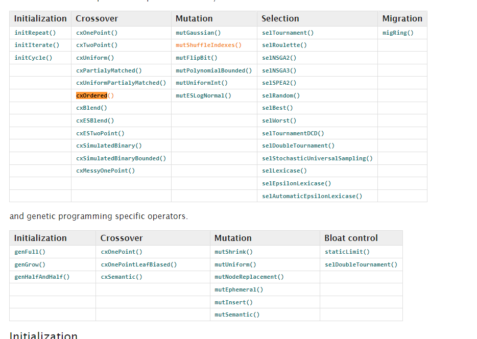
Use cxOrdered crossover and mutationShuffleIndexes mutation.
Note
deap.tools.mutShuffleIndexes(individual, indpb)[source]
Shuffle the attributes of the input individual and return the mutant. The individual is expected to be a sequence. The indpb argument is the probability of each attribute to be moved. Usually this mutation is applied on vector of indices.
deap.tools.cxOrdered(ind1, ind2)[source]
Executes an ordered crossover (OX) on the input individuals. The two individuals are modified in place. This crossover expects sequence individuals of indices, the result for any other type of individuals is unpredictable.
More Operators:
1.4.3.2. Solution#
from deap import base
from deap import creator
from deap import tools
from deap import algorithms

import random
import array

import numpy as np
import matplotlib.pyplot as plt
import seaborn as sns
# set the random seed for repeatable results
RANDOM_SEED = 42
random.seed(RANDOM_SEED)

# create the desired traveling salesman problem instace:
TSP_NAME = "bayg29"  # name of problem
tsp = TravelingSalesmanProblem(TSP_NAME)

# Genetic Algorithm constants:
POPULATION_SIZE = 300
MAX_GENERATIONS = 200
HALL_OF_FAME_SIZE = 1
P_CROSSOVER = 0.9  # probability for crossover
P_MUTATION = 0.1   # probability for mutating an individual

toolbox = base.Toolbox()
# define a single objective, minimizing fitness strategy:
creator.create("FitnessMin", base.Fitness, weights=(-1.0,))

# create the Individual class based on list of integers:
creator.create("Individual", array.array, typecode='i', fitness=creator.FitnessMin)

# create an operator that generates randomly shuffled indices:
toolbox.register("randomOrder", random.sample, range(len(tsp)), len(tsp))

# create the individual creation operator to fill up an Individual instance with shuffled indices:
toolbox.register("individualCreator", tools.initIterate, creator.Individual, toolbox.randomOrder)

# create the population creation operator to generate a list of individuals:
toolbox.register("populationCreator", tools.initRepeat, list, toolbox.individualCreator)
# Calculating The Distance as the TSP Distance.


# fitness calculation - compute the total distance of the list of cities represented by indices:
def tpsDistance(individual):
    return tsp.getTotalDistance(individual),  # return a tuple


toolbox.register("evaluate", tpsDistance)

# Genetic operators:
toolbox.register("select", tools.selTournament, tournsize=3)
toolbox.register("mate", tools.cxOrdered)
toolbox.register("mutate", tools.mutShuffleIndexes, indpb=1.0/len(tsp))
# create initial population (generation 0):
population = toolbox.populationCreator(n=POPULATION_SIZE)

# prepare the statistics object:
stats = tools.Statistics(lambda ind: ind.fitness.values)
stats.register("min", np.min)
stats.register("avg", np.mean)
# define the hall-of-fame object:
hof = tools.HallOfFame(HALL_OF_FAME_SIZE)
# perform the Genetic Algorithm flow with hof feature added:
population, logbook = algorithms.eaSimple(population, toolbox, cxpb=P_CROSSOVER, mutpb=P_MUTATION,
                                            ngen=MAX_GENERATIONS, stats=stats, halloffame=hof, verbose=True)

# print best individual info:
best = hof.items[0]
print("-- Best Ever Individual = ", best)
print("-- Best Ever Fitness = ", best.fitness.values[0])
gen	nevals	min    	avg
0  	300   	21103.3	26457
1  	279   	19562.4	25128.9
2  	275   	19456.5	24267.3
3  	279   	19760.9	23592
4  	278   	19406.4	22963.5
5  	276   	19105.2	22480.7
6  	281   	17802.4	22129.9
7  	279   	18160.2	21581.5
8  	274   	17691.3	21253.6
9  	277   	16011.9	20877.8
10 	268   	16011.9	20597.9
11 	279   	15878.8	20413.2
12 	269   	14589.1	20188.2
13 	272   	14589.1	19987.8
14 	281   	15182.9	19910.4
15 	276   	15836.2	19437
16 	276   	15687.4	19117.2
17 	282   	15426.5	19039.4
18 	282   	14905.2	18696.7
19 	269   	15020.4	18614.9
20 	275   	13346.3	18424
21 	276   	14711.4	18330.1
22 	275   	13139.1	18312
23 	274   	13139.1	18005
24 	278   	13002.5	17725.6
25 	262   	12203.5	17543.2
26 	274   	13157.3	17285.2
27 	260   	12918.6	16946.3
28 	271   	12918.6	16646
29 	262   	12918.6	16441
30 	279   	12652.9	16194.2
31 	265   	12652.9	15910.6
32 	278   	12565.6	15942.4
33 	278   	12520.5	15682
34 	283   	12436.1	15569.5
35 	272   	12214  	15441.9
36 	265   	12278.3	15353.6
37 	271   	12302.9	15371.8
38 	273   	12037.5	15182
39 	271   	11969.4	14974.3
40 	267   	12081.2	14825
41 	266   	11785.8	14612.3
42 	282   	11477  	14591.8
43 	269   	10869.8	14446
44 	270   	11475  	14452.8
45 	277   	11796.8	14491.9
46 	277   	11262.8	14324.7
47 	277   	11333.1	14183.2
48 	281   	11311  	14135.4
49 	271   	10921.8	14212.2
50 	274   	11172.8	14137.9
51 	279   	11295.1	13945
52 	280   	10870.6	14044.3
53 	278   	11225.2	14167.9
54 	270   	11336.3	13993.6
55 	268   	10472.9	13886.4
56 	285   	10637.9	13841.5
57 	285   	10885.9	13732.8
58 	273   	10885.9	13634.4
59 	277   	10885.9	13478.8
60 	265   	10835.7	13253.8
61 	264   	10526.5	13286.8
62 	268   	10445.5	12951.3
63 	276   	10501.6	12833.3
64 	267   	10484.8	12683.7
65 	280   	10501.6	12505
66 	277   	10355.2	12469.2
67 	268   	10231.6	12586.4
68 	273   	10367.5	12436.2
69 	281   	10355.2	12450.7
70 	274   	10281.8	12607.8
71 	261   	10281.8	12339.2
72 	269   	10163.3	12328.2
73 	276   	10048.3	12238.8
74 	272   	10048.3	12162.9
75 	270   	10029.8	12178.7
76 	273   	9957.92	12117
77 	272   	9957.92	12131.7
78 	276   	9852.51	11973.6
79 	273   	9852.51	11883.2
80 	268   	9775.74	11853.7
81 	288   	9775.74	11715.1
82 	276   	9775.74	11806.3
83 	276   	9775.74	11826.1
84 	268   	9775.74	11618.9
85 	271   	9775.74	11430.3
86 	265   	9775.74	11586.3
87 	269   	9775.74	11394.7
88 	259   	9775.74	11172.9
89 	275   	9775.74	11210.5
90 	275   	9775.74	11081.7
91 	272   	9775.74	11051.4
92 	277   	9775.74	11065
93 	274   	9775.74	11113.7
94 	276   	9775.74	11010
95 	272   	9775.74	10886.1
96 	272   	9771.1 	10758.8
97 	267   	9771.1 	10639.7
98 	279   	9771.1 	10681.8
99 	262   	9771.1 	10511.1
100	279   	9771.1 	10403.5
101	284   	9771.1 	10424.7
102	275   	9767.79	10432.8
103	266   	9767.79	10418
104	272   	9767.79	10264.2
105	285   	9767.79	10185.9
106	277   	9767.79	10167.7
107	279   	9767.79	10131.7
108	269   	9763.16	10109.5
109	273   	9734.57	10126.7
110	282   	9729.93	10360.6
111	268   	9729.93	10356.4
112	272   	9729.93	10529.1
113	271   	9729.93	10511.3
114	275   	9729.93	10510.6
115	270   	9729.93	10166.8
116	280   	9729.93	10064.7
117	257   	9729.93	9985.98
118	273   	9729.93	9935.52
119	281   	9729.93	9893.57
120	268   	9729.93	9936.33
121	282   	9729.93	10072.7
122	285   	9729.93	9927.8
123	270   	9729.93	9995.76
124	266   	9729.93	9932.75
125	274   	9729.93	9938.32
126	284   	9729.93	9972.79
127	263   	9616.16	9979.21
128	275   	9616.16	9910.33
129	277   	9616.16	9975.06
130	272   	9616.16	10001.9
131	279   	9616.16	9999.09
132	284   	9616.16	9969.31
133	271   	9616.16	9917.73
134	262   	9616.16	9953.55
135	273   	9616.16	9877.65
136	266   	9616.16	9874.04
137	256   	9616.16	9737.42
138	274   	9616.16	9825.19
139	272   	9616.16	9901.44
140	269   	9616.16	9846.18
141	266   	9558.06	9843.06
142	263   	9558.06	9804.26
143	261   	9558.06	9871.85
144	279   	9558.06	9829.84
145	273   	9558.06	9939.57
146	268   	9558.06	9771.86
147	278   	9558.06	9779.87
148	278   	9556.72	9787.78
149	281   	9549.99	9779
150	272   	9549.99	9803.48
151	278   	9549.99	9809.74
152	270   	9549.99	9780.88
153	271   	9549.99	9686.82
154	269   	9549.99	9880.91
155	265   	9549.99	9899.8
156	282   	9549.99	9978.31
157	277   	9549.99	9823.43
158	273   	9549.99	10009.3
159	279   	9549.99	9954.48
160	273   	9549.99	9980.84
161	273   	9549.99	9985.32
162	282   	9549.99	9923.51
163	284   	9549.99	9981.25
164	273   	9549.99	10222.2
165	263   	9549.99	10151
166	271   	9549.99	10154.6
167	279   	9549.99	10073.1
168	267   	9549.99	9895.51
169	277   	9549.99	9781.48
170	270   	9549.99	9840.1
171	273   	9549.99	9744.42
172	273   	9549.99	9811.11
173	277   	9549.99	9792.8
174	284   	9549.99	9860.57
175	273   	9549.99	9668.35
176	266   	9549.99	9705.16
177	275   	9549.99	9800.14
178	270   	9549.99	9751.82
179	281   	9549.99	9816.48
180	269   	9549.99	9743.48
181	280   	9549.99	9715.93
182	278   	9549.99	9792.3
183	280   	9549.99	9716.09
184	290   	9549.99	9811.45
185	281   	9549.99	9758.04
186	269   	9549.99	9693.11
187	281   	9549.99	9761.23
188	273   	9549.99	9712.46
189	262   	9549.99	9786.26
190	276   	9549.99	9805.2
191	282   	9549.99	9675.81
192	269   	9549.99	9733.11
193 258 9549.99 9981.48
194 273 9549.99 9722.19
195 267 9549.99 9694.95
196 281 9549.99 9845.83
197 262 9549.99 9903.02
198 274 9549.99 9749.83
199 270 9549.99 9886.32
200 277 9549.99 9837.95
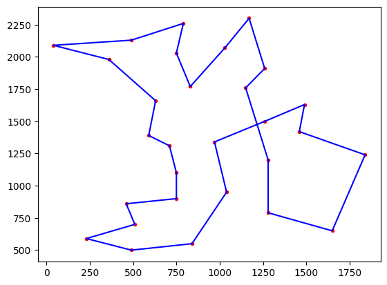
-- Best Ever Individual = Individual('i', [0, 27, 11, 5, 20, 4, 8, 25, 2, 28, 1, 19, 9, 3, 14, 17, 13, 16, 21, 10, 18, 12, 23, 7, 26, 22, 6, 24, 15])
-- Best Ever Fitness = 9549.9853515625
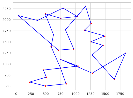
# plot best solution:
plt.figure(1)
tsp.plotData(best)
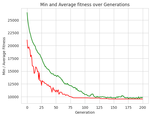
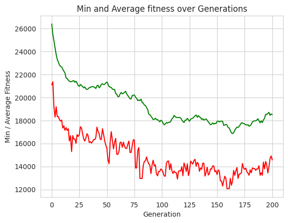
# plot statistics:
minFitnessValues, meanFitnessValues = logbook.select("min", "avg")
plt.figure(2)
sns.set_style("whitegrid")
plt.plot(minFitnessValues, color='red')
plt.plot(meanFitnessValues, color='green')
plt.xlabel('Generation')
plt.ylabel('Min / Average Fitness')
plt.title('Min and Average fitness over Generations')
# show both plots:
plt.show()
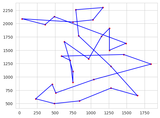
1.4.4. TSP Modifying Tour Size: 3#
Experimenting with the Tournament Size reveals that: When the size is increasing the size of the torunament, is not able to retain the best solutions…
# Calculating The Distance as the TSP Distance.


# fitness calculation - compute the total distance of the list of cities represented by indices:
def tpsDistance(individual):
    return tsp.getTotalDistance(individual),  # return a tuple


toolbox.register("evaluate", tpsDistance)


# Genetic operators:
toolbox.register("select", tools.selTournament, tournsize=2)
toolbox.register("mate", tools.cxOrdered)
toolbox.register("mutate", tools.mutShuffleIndexes, indpb=1.0/len(tsp))

# create initial population (generation 0):
population = toolbox.populationCreator(n=POPULATION_SIZE)

# prepare the statistics object:
stats = tools.Statistics(lambda ind: ind.fitness.values)
stats.register("min", np.min)
stats.register("avg", np.mean)


# define the hall-of-fame object:
hof = tools.HallOfFame(HALL_OF_FAME_SIZE)

# perform the Genetic Algorithm flow with hof feature added:
population, logbook = algorithms.eaSimple(population, toolbox, cxpb=P_CROSSOVER, mutpb=P_MUTATION,
                                            ngen=MAX_GENERATIONS, stats=stats, halloffame=hof, verbose=True)

# print best individual info:
best = hof.items[0]
print("-- Best Ever Individual = ", best)
print("-- Best Ever Fitness = ", best.fitness.values[0])
gen	nevals	min    	avg
0  	300   	21103.5	26399.8
1  	274   	21361.6	25481.4
2  	258   	19153.7	24928.2
3  	285   	18299.3	24318.2
4  	275   	19199.8	23753.1
5  	271   	18344.1	23313.5
6  	270   	18344.1	23081.9
7  	264   	18078.7	22838.6
8  	273   	17945.4	22705.6
9  	276   	18042.5	22653.7
10 	263   	17340.4	22467.2
11 	268   	17549.7	22291.7
12 	272   	17144.4	22138.2
13 	274   	17379.9	21704.1
14 	269   	17143.3	21659.2
15 	261   	17288.3	21517.3
16 	273   	16224.5	21419.9
17 	277   	16676.9	21367.1
18 	263   	15293  	21390.3
19 	272   	16688.3	21436.5
20 	272   	16388.9	21475.2
21 	270   	16388.9	21326.1
22 	278   	16014.6	21420.9
23 	273   	16779.1	21255.7
24 	278   	16615  	21044
25 	254   	16738.1	20971.9
26 	274   	17463  	21139.5
27 	274   	17331.4	21043.8
28 	272   	16859.7	20956.5
29 	271   	16402  	20855
30 	271   	16206.3	20919.5
31 	271   	16492.5	20749.2
32 	268   	16853.3	20707.1
33 	264   	16667.7	20748.3
34 	288   	16083.8	20855.3
35 	277   	16157.7	20896.1
36 	265   	16036.8	20924.3
37 	266   	16169.1	20953.2
38 	268   	16335.5	20932.7
39 	279   	16335.5	20877.3
40 	269   	16521.9	20784.1
41 	281   	17424.2	21013.6
42 	273   	17046.1	21073.9
43 	262   	16854  	20843.3
44 	276   	16357.8	20953.5
45 	276   	16357.8	21156
46 	265   	17285.9	21187.9
47 	276   	16799.8	21134.7
48 	277   	16251  	21150.8
49 	272   	15854.7	21271.9
50 	277   	15588.8	21348.2
51 	278   	14563.7	21173.6
52 	279   	14249.4	20943.6
53 	265   	16149.7	20917.3
54 	275   	17031.8	20867.9
55 	274   	16278.2	20746.1
56 	262   	15532.3	20685.8
57 	267   	16097.3	20703.7
58 	277   	16441.2	20357.1
59 	285   	15057.9	20287
60 	270   	15057.9	20072.7
61 	263   	15311.8	20077.8
62 	275   	16103.8	20311.4
63 	270   	16103.8	20438.1
64 	274   	15672.4	20323.6
65 	268   	16123.5	20361.7
66 	258   	15764.1	20453.8
67 	278   	15573.2	20546.5
68 	278   	15573.2	20312.7
69 	276   	15945  	20168.7
70 	262   	16211  	20045.8
71 	265   	15224.5	19886.9
72 	275   	15224.5	19888.3
73 	280   	15809  	20169.8
74 	278   	16331.9	20202
75 	271   	16285.4	20218.7
76 	268   	13871.3	20027.3
77 	264   	13871.3	19940.9
78 	264   	15407  	19734.6
79 	267   	15645.2	19789.4
80 	276   	12955.5	19732.4
81 	272   	12955.5	19861.2
82 	273   	12955.5	19564.4
83 	268   	14070.9	19513.9
84 	271   	14445.9	19350.3
85 	281   	14502.3	19297.6
86 	278   	14827.2	19126.1
87 	268   	14461.4	18970.9
88 	255   	14230.7	18559.6
89 	270   	14109.2	18499.4
90 	265   	13381.8	18369.5
91 	272   	14131.6	18252
92 	275   	14549.2	18079.1
93 	273   	14048.4	18096.7
94 	284   	14137.4	18202.6
95 	258   	13344.2	18079.2
96 	274   	13191  	18065.4
97 	276   	13570.1	18014.6
98 	272   	13570.1	17879.5
99 	277   	13789.3	18022
100	280   	13691.4	17954.3
101	274   	13468.1	17759.1
102	280   	13172.8	17626.5
103	268   	13159.3	17696.3
104	259   	14291  	17820
105	279   	14462.7	17779.8
106	265   	14476.2	17836
107	268   	13715.8	17840.7
108	276   	14242.1	17942.9
109	284   	13628  	18132.7
110	273   	13390.5	18238.5
111	279   	13600.3	18442.6
112	266   	13461.5	18331.3
113	271   	13461.5	18271.2
114	280   	12910.8	18261.2
115	281   	13587.4	18260.8
116	269   	13639.6	18263.5
117	273   	13603.5	18210.9
118	276   	13977.8	18051.2
119	280   	13195.3	17917.1
120	273   	14310.7	17827.5
121	262   	13982.4	18028.4
122	273   	13569.9	18039.5
123	278   	14228.8	18189.9
124	276   	13208.5	18056.2
125	265   	13632.2	17937.3
126	273   	14468.8	18115.5
127	274   	14330.4	18172.6
128	268   	14212.1	18202.2
129	282   	14523.6	18310.7
130	280   	14624.1	18408.5
131	277   	14025.1	18482.2
132	279   	14359.8	18284.9
133	270   	14243.4	18428.7
134	273   	13577  	18301.5
135	282   	13878.6	18267.4
136	268   	13758.6	18087.1
137	270   	14297.1	18154.7
138	268   	14274.6	18039.8
139	285   	13162.2	18088.6
140	281   	13472.2	18132.5
141	266   	13937.4	18021.2
142	267   	13257.5	17882.7
143	266   	13376.4	17756.5
144	277   	13796.6	17633.3
145	278   	13769.7	17685.6
146	276   	14044.2	17795.6
147	267   	14044.2	17691.6
148	270   	13542.7	17753.6
149	264   	13634.8	17730.1
150	276   	13294.7	17928.2
151	276   	13693.6	17949.9
152	277   	13600.8	17875.5
153	274   	12738.6	17938.5
154	268   	12738.6	17944
155	273   	12296.6	17932.7
156	269   	12741.2	17570.3
157	274   	13152.3	17612.7
158	273   	12946  	17662.3
159	264   	12070.9	17603.5
160	267   	12070.9	17389.9
161	264   	12070.9	17347.1
162	279   	12967.3	17124
163	275   	12370.7	16920
164	274   	12730.9	16864.2
165	270   	13658.8	16925.7
166	267   	13225.9	17144.9
167	267   	13610.7	17313.1
168	276   	13912.6	17418.3
169	270   	12961.4	17399.4
170	271   	13335.9	17502.1
171	273   	13357.5	17628.6
172	263   	13456.1	17795.4
173	275   	14259.9	17795.4
174	267   	13859.9	17726.7
175	269   	13752  	17703.6
176	269   	13852.9	17626.9
177	283   	13539  	17612.7
178	273   	13418.4	17636.9
179	262   	13230.4	17498.5
180	279   	13702  	17553.1
181	279   	13456.2	17665
182	270   	13874.4	17881.2
183	280   	13818.4	17950.4
184	271   	13818.4	17969.7
185	279   	13660.9	17971.5
186	272   	13793.1	18030.4
187	265   	13793.1	18153.7
188	286   	14066.1	17980.3
189	258   	13236.8	17798.1
190	272   	13463.7	17976.3
191	277   	13233.5	17818.7
192	276   	14378.3	18048.2
193	271   	13784.3	18182.4
194	278   	14436.5	18534.6
195	277   	14171.8	18530.7
196	281   	13440.1	18614.7
197	273   	13938.8	18707.3
198	271   	14678.1	18458
199	271   	14921.4	18568.2
200	258   	14572.3	18512.5
-- Best Ever Individual =  Individual('i', [11, 27, 0, 7, 23, 26, 15, 6, 22, 24, 3, 18, 17, 13, 16, 21, 10, 14, 19, 1, 25, 4, 5, 8, 28, 2, 9, 12, 20])
-- Best Ever Fitness =  12070.9267578125
# plot best solution:
plt.figure(1)
tsp.plotData(best)
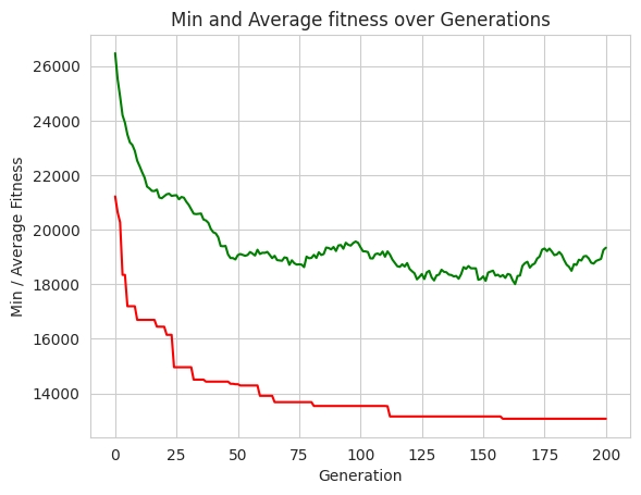
# plot statistics:
minFitnessValues, meanFitnessValues = logbook.select("min", "avg")
plt.figure(2)
sns.set_style("whitegrid")
plt.plot(minFitnessValues, color='red')
plt.plot(meanFitnessValues, color='green')
plt.xlabel('Generation')
plt.ylabel('Min / Average Fitness')
plt.title('Min and Average fitness over Generations')
# show both plots:
plt.show()
### Attempt using Elitism

import elitism

# Calculating The Distance as the TSP Distance.


# fitness calculation - compute the total distance of the list of cities represented by indices:
def tpsDistance(individual):
    return tsp.getTotalDistance(individual),  # return a tuple


toolbox.register("evaluate", tpsDistance)


# Genetic operators:
toolbox.register("select", tools.selTournament, tournsize=2)
toolbox.register("mate", tools.cxOrdered)
toolbox.register("mutate", tools.mutShuffleIndexes, indpb=1.0/len(tsp))

# create initial population (generation 0):
population = toolbox.populationCreator(n=POPULATION_SIZE)

# prepare the statistics object:
stats = tools.Statistics(lambda ind: ind.fitness.values)
stats.register("min", np.min)
stats.register("avg", np.mean)


# define the hall-of-fame object:
hof = tools.HallOfFame(HALL_OF_FAME_SIZE)

# perform the Genetic Algorithm flow with hof feature added:
# population, logbook = algorithms.eaSimple(population, toolbox, cxpb=P_CROSSOVER, mutpb=P_MUTATION,
#                                             ngen=MAX_GENERATIONS, stats=stats, halloffame=hof, verbose=True)

population, logbook = elitism.eaSimpleWithElitism(population, toolbox, cxpb=P_CROSSOVER, mutpb=P_MUTATION,
                                            ngen=MAX_GENERATIONS, stats=stats, halloffame=hof, verbose=True)


# print best individual info:
best = hof.items[0]
print("-- Best Ever Individual = ", best)
print("-- Best Ever Fitness = ", best.fitness.values[0])


# plot best solution:
plt.figure(1)
tsp.plotData(best)

# plot statistics:
minFitnessValues, meanFitnessValues = logbook.select("min", "avg")
plt.figure(2)
sns.set_style("whitegrid")
plt.plot(minFitnessValues, color='red')
plt.plot(meanFitnessValues, color='green')
plt.xlabel('Generation')
plt.ylabel('Min / Average Fitness')
plt.title('Min and Average fitness over Generations')

# show both plots:
plt.show()
gen	nevals	min    	avg
0  	300   	21219.9	26467.8
1  	276   	20638  	25521.8
2  	282   	20272.5	24884.4
3  	260   	18344.9	24197.1
4  	278   	18344.9	23918.4
5  	278   	17194.8	23487.6
6  	280   	17194.8	23202.3
7  	282   	17194.8	23106
8  	275   	17194.8	22890.5
9  	278   	16695.1	22527.2
10 	273   	16695.1	22323.1
11 	279   	16695.1	22103
12 	275   	16695.1	21905.8
13 	262   	16695.1	21578.5
14 	270   	16695.1	21511.8
15 	271   	16695.1	21421.8
16 	267   	16695.1	21416.1
17 	269   	16448.3	21469.7
18 	271   	16443.9	21180.3
19 	278   	16443.9	21154.2
20 	282   	16443.9	21224.8
21 	273   	16147.2	21298.1
22 	275   	16147.2	21319.3
23 	270   	16147.2	21238.5
24 	277   	14959.4	21254.6
25 	269   	14959.4	21262.3
26 	272   	14959.4	21114.6
27 	260   	14959.4	21199.2
28 	280   	14959.4	21174
29 	270   	14959.4	21024.7
30 	271   	14959.4	20909.9
31 	267   	14959.4	20744
32 	270   	14505.1	20586.8
33 	276   	14505.1	20572.7
34 	268   	14505.1	20585.1
35 	277   	14505.1	20593.3
36 	273   	14505.1	20373.2
37 	269   	14432.1	20338.1
38 	265   	14432.1	20251.1
39 	270   	14432.1	20027
40 	268   	14432.1	19904.4
41 	270   	14432.1	19865.6
42 	281   	14432.1	19723.6
43 	272   	14432.1	19403.4
44 	263   	14432.1	19393.1
45 	279   	14432.1	19404.7
46 	278   	14432.1	19095
47 	265   	14353.2	18961
48 	279   	14353.2	18960.3
49 	272   	14336.5	18909.9
50 	279   	14336.5	19068.2
51 	266   	14291  	19109.2
52 	260   	14291  	19077.7
53 	267   	14291  	19043.8
54 	278   	14291  	19074.8
55 	270   	14291  	19183
56 	263   	14291  	19122.6
57 	276   	14291  	19053.9
58 	280   	14291  	19265
59 	268   	13912.2	19110.3
60 	280   	13912.2	19154.2
61 	274   	13912.2	19151.5
62 	279   	13912.2	19186.3
63 	274   	13912.2	19076.5
64 	270   	13912.2	18957
65 	271   	13680  	19043.5
66 	268   	13680  	18885.5
67 	275   	13680  	18870.7
68 	282   	13680  	18860.3
69 	281   	13680  	18984.5
70 	275   	13680  	18966
71 	275   	13680  	18713.1
72 	270   	13680  	18877.2
73 	267   	13680  	18771.1
74 	276   	13680  	18721.6
75 	272   	13680  	18730.5
76 	274   	13680  	18719.6
77 	280   	13680  	18629.1
78 	271   	13680  	19013.3
79 	276   	13680  	18954.8
80 	263   	13680  	18965.8
81 	268   	13539.2	19078.7
82 	269   	13539.2	18964.2
83 	269   	13539.2	19171.5
84 	263   	13539.2	19073.9
85 	273   	13539.2	19108.6
86 	270   	13539.2	19345.2
87 	266   	13539.2	19330.6
88 	260   	13539.2	19278.1
89 	272   	13539.2	19367.2
90 	276   	13539.2	19219
91 	271   	13539.2	19422
92 	269   	13539.2	19438.4
93 	271   	13539.2	19301.6
94 	281   	13539.2	19521.6
95 	267   	13539.2	19447
96 	267   	13539.2	19416.6
97 	276   	13539.2	19510.2
98 	281   	13539.2	19566.9
99 	265   	13539.2	19519.1
100	267   	13539.2	19356.7
101	264   	13539.2	19210.5
102	273   	13539.2	19203.6
103	277   	13539.2	19181.4
104	267   	13539.2	18950.4
105	270   	13539.2	18946.4
106	277   	13539.2	19101.3
107	278   	13539.2	19126.7
108	277   	13539.2	19076.7
109	270   	13539.2	19198.5
110	260   	13539.2	19010.5
111	265   	13531.3	19203.9
112	276   	13155.3	19083.3
113	283   	13155.3	18903.2
114	271   	13155.3	18779.2
115	280   	13155.3	18662
116	279   	13155.3	18638.1
117	266   	13155.3	18731.5
118	267   	13155.3	18649.7
119	272   	13155.3	18777.7
120	276   	13155.3	18563.6
121	271   	13155.3	18477.8
122	266   	13155.3	18401.6
123	284   	13155.3	18180.6
124	279   	13155.3	18271
125	267   	13155.3	18375.8
126	283   	13155.3	18192
127	264   	13155.3	18437.5
128	276   	13155.3	18491.9
129	250   	13155.3	18249.9
130	267   	13155.3	18140
131	267   	13155.3	18326
132	271   	13155.3	18352.6
133	273   	13155.3	18533
134	273   	13155.3	18456.4
135	271   	13155.3	18440.1
136	275   	13155.3	18353.6
137	273   	13155.3	18340.5
138	274   	13155.3	18287.8
139	276   	13155.3	18304.6
140	272   	13155.3	18203.1
141	278   	13155.3	18367.2
142	273   	13155.3	18628.6
143	264   	13155.3	18564.2
144	278   	13155.3	18668
145	260   	13155.3	18585.9
146	276   	13155.3	18586.5
147	263   	13155.3	18583.1
148	270   	13155.3	18165.6
149	270   	13155.3	18193.8
150	262   	13155.3	18288.4
151	272   	13155.3	18125.1
152	274   	13155.3	18429.8
153	259   	13155.3	18464
154	265   	13155.3	18499.6
155	269   	13155.3	18317.6
156	286   	13155.3	18350.5
157	255   	13155.3	18277.5
158	274   	13071  	18338.9
159	269   	13071  	18233.7
160	267   	13071  	18378
161	273   	13071  	18350.4
162	282   	13071  	18146.3
163	274   	13071  	18005.8
164	279   	13071  	18303.3
165	273   	13071  	18319.4
166	285   	13071  	18674.4
167	276   	13071  	18771.8
168	266   	13071  	18825.1
169	255   	13071  	18610.6
170	275   	13071  	18712.8
171	271   	13071  	18762.3
172	267   	13071  	18941.9
173	284   	13071  	19018.1
174	274   	13071  	19268.8
175	274   	13071  	19311.6
176	266   	13071  	19214.6
177	281   	13071  	19308.3
178	289   	13071  	19196.7
179	277   	13071  	19067.4
180	256   	13071  	19091.8
181	286   	13071  	19183.3
182	270   	13071  	19080.7
183	269   	13071  	18880.7
184	262   	13071  	18716.6
185	265   	13071  	18638.1
186	277   	13071  	18493.9
187	275   	13071  	18739.1
188	267   	13071  	18706.8
189	266   	13071  	18900.2
190	271   	13071  	18870
191	282   	13071  	19022.7
192	268   	13071  	19037.4
193	274   	13071  	18949
194	263   	13071  	18789
195	275   	13071  	18757.7
196	272   	13071  	18854.2
197	259   	13071  	18893.6
198	273   	13071  	18928.7
199	265   	13071  	19257.7
200	280   	13071  	19339.1
-- Best Ever Individual =  Individual('i', [13, 17, 16, 21, 10, 24, 6, 15, 20, 8, 11, 5, 4, 2, 28, 25, 7, 23, 27, 0, 12, 1, 3, 14, 9, 19, 26, 22, 18])
-- Best Ever Fitness =  13071.04296875
from deap import base
from deap import creator
from deap import tools
import random
import array
import numpy as np
import matplotlib.pyplot as plt
import seaborn as sns
import tsp
import elitism
# set the random seed for repeatable results
RANDOM_SEED = 42
random.seed(RANDOM_SEED)
# create the desired traveling salesman problem instace:
TSP_NAME = "bayg29" # name of problem
tsp = tsp.TravelingSalesmanProblem(TSP_NAME)
# Genetic Algorithm constants:
POPULATION_SIZE = 300
MAX_GENERATIONS = 200
HALL_OF_FAME_SIZE = 30
P_CROSSOVER = 0.9 # probability for crossover
P_MUTATION = 0.1 # probability for mutating an individual
toolbox = base.Toolbox()
# define a single objective, minimizing fitness strategy:
creator.create("FitnessMin", base.Fitness, weights=(-1.0,))
# create the Individual class based on list of integers:
creator.create("Individual", array.array, typecode='i', fitness=creator.FitnessMin)
# create an operator that generates randomly shuffled indices:
toolbox.register("randomOrder", random.sample, range(len(tsp)), len(tsp))
# create the individual creation operator to fill up an Individual instance with shuffled indices:
toolbox.register("individualCreator", tools.initIterate, creator.Individual, toolbox.randomOrder)
# create the population creation operator to generate a list of individuals:
toolbox.register("populationCreator", tools.initRepeat, list, toolbox.individualCreator)
# fitness calculation - compute the total distance of the list of cities represented by indices:
def tpsDistance(individual):
return tsp.getTotalDistance(individual), # return a tuple
toolbox.register("evaluate", tpsDistance)
# Genetic operators:
toolbox.register("select", tools.selTournament, tournsize=2)
toolbox.register("mate", tools.cxOrdered)
toolbox.register("mutate", tools.mutShuffleIndexes, indpb=1.0/len(tsp))
# create initial population (generation 0):
population = toolbox.populationCreator(n=POPULATION_SIZE)
# prepare the statistics object:
stats = tools.Statistics(lambda ind: ind.fitness.values)
stats.register("min", np.min)
stats.register("avg", np.mean)
# define the hall-of-fame object:
hof = tools.HallOfFame(HALL_OF_FAME_SIZE)
# perform the Genetic Algorithm flow with hof feature added:
population, logbook = elitism.eaSimpleWithElitism(population, toolbox, cxpb=P_CROSSOVER, mutpb=P_MUTATION,
ngen=MAX_GENERATIONS, stats=stats, halloffame=hof, verbose=True)
# print best individual info:
best = hof.items[0]
print("-- Best Ever Individual = ", best)
print("-- Best Ever Fitness = ", best.fitness.values[0])
# plot best solution:
plt.figure(1)
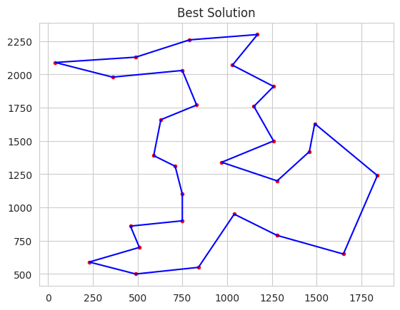
tsp.plotData(best, label='Best Solution')
# plot statistics:
minFitnessValues, meanFitnessValues = logbook.select("min", "avg")
plt.figure(2)
sns.set_style("whitegrid")
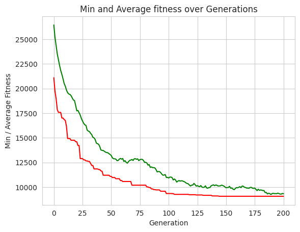
plt.plot(minFitnessValues, color='red')
plt.plot(meanFitnessValues, color='green')
plt.xlabel('Generation')
plt.ylabel('Min / Average Fitness')
plt.title('Min and Average fitness over Generations')
# show both plots:
plt.show()
gen	nevals	min    	avg
0  	300   	21103.3	26457
1  	252   	19726.4	25210.9
2  	249   	18977.1	24364.3
3  	257   	17868.2	23514.7
4  	237   	17585.3	22929.8
5  	247   	17585.3	22350.6
6  	247   	17585.3	21831.4
7  	249   	17012.3	21442.6
8  	238   	17012.3	20999.7
9  	249   	16856.3	20513.2
10 	249   	16766.4	20235.4
11 	249   	16165.7	19852.8
12 	244   	14934  	19588.4
13 	242   	14934  	19454.3
14 	252   	14934  	19412.6
15 	245   	14757.5	19286.6
16 	242   	14757.5	19057.2
17 	253   	14757.5	18846.9
18 	246   	14757.5	18782.7
19 	240   	14607  	18293.7
20 	249   	14607  	17740.2
21 	248   	14227.7	17786.1
22 	238   	14227.7	17546.7
23 	242   	12893.9	17310.7
24 	245   	12893.9	16959.3
25 	241   	12893.9	16699.8
26 	242   	12766.2	16481.4
27 	246   	12766.2	16321.5
28 	246   	12662.4	16263.8
29 	236   	12662.4	15799.7
30 	248   	12610.1	15691.9
31 	245   	12610.1	15636.5
32 	247   	12410.6	15465
33 	253   	12199.6	15328.7
34 	242   	12199.6	15059.9
35 	237   	11848.8	15000.8
36 	251   	11848.8	14836.8
37 	237   	11848.8	14476.5
38 	240   	11848.8	14406.1
39 	251   	11787.9	14350.9
40 	244   	11787.9	14119.6
41 	240   	11645.8	13769.5
42 	248   	11611.2	13731.4
43 	251   	11208.4	13714.4
44 	243   	11208.4	13642.7
45 	245   	11208.4	13548.5
46 	256   	11208.4	13507.2
47 	247   	11208.4	13489.6
48 	244   	11208.4	13402.3
49 	240   	11093.4	13304.7
50 	248   	11093.4	13213.2
51 	241   	10975.6	12976.7
52 	235   	10975.6	12877.5
53 	257   	10975.6	12878.6
54 	247   	10855.3	12847
55 	246   	10855.3	12690
56 	245   	10855.3	12702.2
57 	246   	10855.3	12835.6
58 	251   	10673.6	12916
59 	248   	10673.6	12836.2
60 	240   	10572.8	12905.9
61 	230   	10572.8	12600.5
62 	245   	10572.8	12687.6
63 	253   	10572.8	12515.9
64 	235   	10572.8	12429
65 	245   	10572.8	12582.2
66 	232   	10572.8	12713.7
67 	252   	10572.8	12741.4
68 	235   	10197.1	12809.4
69 	244   	10197.1	12705.1
70 	257   	10197.1	12876.2
71 	247   	10197.1	12885.3
72 	254   	10197.1	12819.5
73 	242   	10197.1	12871.6
74 	233   	10197.1	12692.1
75 	243   	10197.1	12795.3
76 	242   	10197.1	12824.4
77 	246   	10197.1	12819.1
78 	239   	10197.1	12716.5
79 	246   	10197.1	12514.2
80 	238   	10197.1	12521.6
81 	245   	10021.4	12453.3
82 	252   	10021.4	12233.4
83 	251   	9958.81	12295.2
84 	246   	9958.81	12005.7
85 	243   	9817.91	12051.9
86 	239   	9817.91	11983.5
87 	253   	9752.08	11980.8
88 	243   	9752.08	11948.1
89 	232   	9718.78	11783.5
90 	244   	9718.78	11544.6
91 	253   	9718.78	11590.4
92 	248   	9718.78	11575.3
93 	246   	9584.21	11487.4
94 	237   	9584.21	11324.7
95 	237   	9584.21	11209.5
96 	244   	9584.21	11226.7
97 	257   	9584.21	11277.8
98 	238   	9352.51	10975
99 	249   	9352.51	10994.3
100	236   	9352.51	10923.4
101	250   	9352.51	11018.6
102	242   	9352.51	11023.7
103	254   	9341.54	10962.8
104	241   	9341.54	10727.6
105	241   	9266.7 	10828.5
106	236   	9266.7 	10722.4
107	246   	9266.7 	10516.8
108	246   	9266.69	10608.1
109	243   	9266.69	10671
110	243   	9266.69	10615.1
111	255   	9266.69	10645
112	246   	9266.69	10633.7
113	252   	9266.69	10576.4
114	243   	9266.69	10533.5
115	242   	9266.69	10431.7
116	244   	9266.69	10376.1
117	240   	9266.69	10343.1
118	254   	9232.07	10219.5
119	245   	9232.07	10117.4
120	256   	9232.07	10202.2
121	242   	9232.07	10209.1
122	248   	9232.07	10382
123	246   	9232.07	10256
124	245   	9204.93	10105
125	234   	9204.93	10150.4
126	236   	9204.93	10088.2
127	229   	9204.93	10045.4
128	253   	9204.93	10161.8
129	247   	9204.93	10007
130	246   	9170.3 	9969.34
131	236   	9170.3 	9993.64
132	260   	9170.3 	10131.6
133	242   	9170.3 	9926.74
134	247   	9170.3 	9887.23
135	250   	9170.3 	9966.44
136	243   	9170.3 	9958.18
137	251   	9170.3 	10143.4
138	244   	9108.77	10185.9
139	245   	9108.77	10237.1
140	235   	9108.77	10149.8
141	254   	9108.77	10217.6
142	252   	9104.36	10189.9
143	245   	9104.36	10114.9
144	250   	9074.15	10124.3
145	251   	9074.15	10127.8
146	242   	9074.15	10201.5
147	251   	9074.15	10169.5
148	250   	9074.15	10113.9
149	229   	9074.15	10025.9
150	242   	9074.15	9933.94
151	231   	9074.15	9967.2
152	253   	9074.15	9962.38
153	252   	9074.15	10085.3
154	243   	9074.15	9887.07
155	244   	9074.15	9916.6
156	235   	9074.15	9798.14
157	238   	9074.15	9741.92
158	245   	9074.15	9854.62
159	252   	9074.15	9950.48
160	238   	9074.15	9933.46
161	251   	9074.15	9986.24
162	244   	9074.15	10045.3
163	241   	9074.15	9945.64
164	244   	9074.15	10113
165	244   	9074.15	10091.2
166	252   	9074.15	9984.51
167	246   	9074.15	9963.11
168	245   	9074.15	9903
169	257   	9074.15	9911.7
170	247   	9074.15	9881.34
171	236   	9074.15	9973.72
172	241   	9074.15	9980.26
173	242   	9074.15	9883.92
174	249   	9074.15	9878.07
175	239   	9074.15	9900.23
176	240   	9074.15	9790.76
177	244   	9074.15	9647.22
178	248   	9074.15	9791.55
179	251   	9074.15	9679.68
180	251   	9074.15	9715.82
181	249   	9074.15	9696.82
182	249   	9074.15	9653.68
183	252   	9074.15	9655.67
184	233   	9074.15	9450.34
185	243   	9074.15	9464.17
186	236   	9074.15	9307.74
187	244   	9074.15	9380
188	250   	9074.15	9348.07
189	238   	9074.15	9256.05
190	250   	9074.15	9340.67
191	233   	9074.15	9372.6
192	243   	9074.15	9339.89
193	251   	9074.15	9346.98
194	239   	9074.15	9332.73
195	229   	9074.15	9388.14
196	254   	9074.15	9352.36
197	253   	9074.15	9299.68
198	256   	9074.15	9293.32
199	255   	9074.15	9356.17
200	235   	9074.15	9328.94
-- Best Ever Individual =  Individual('i', [0, 23, 12, 15, 26, 7, 22, 6, 24, 18, 10, 21, 16, 13, 17, 14, 3, 9, 19, 1, 20, 4, 28, 2, 25, 8, 11, 5, 27])
-- Best Ever Fitness =  9074.146484375